Transforming Text Classification with Semantic Search Techniques — Faiss
Classification models serve as supervised tools for organising documents into specific categories. Semantic search emerges as a practical solution for managing new categories and scaling up seamlessly to huge data. Its capability to integrate additional information without extensive retraining adds to its straightforward and reliable nature. Utilizing a nearest neighbors approach, semantic search robustly tackles imbalances in data distribution, ensuring resilient classification across diverse datasets. This adaptability, paired with Faiss library’s advanced capabilities, underscores the transformative potential of semantic search in reshaping the classification landscape. Further, its flexibility strikes a balance between computational efficiency and the evolving nature of datasets.
Implementation of classification models involves two primary approaches: utilizing pre-trained models or training models from scratch/fine-tuning existing ones. Pre-trained models have been trained on a large dataset for a general task which can be fine-tuned for a specific application / task or used directly by loading the model. In contrast, training a model from scratch involves building and training an artificial intelligence model without relying on pre-existing weights or knowledge. Each method comes with its own set of limitations. While pre-trained models offer convenience, they may not always be optimal as the training data might differ from our specific dataset. On the other hand, training models from scratch or fine-tuning requires a substantial amount of data and resources to generate meaningful results. Additionally, both models need re-training if new categories emerge.
In this blog post, we will begin by highlighting the advantages of adopting a semantic search approach. We will then delve into an exploration of Faiss, elucidating its different index types. To illustrate the practical application of this approach, we will walk through a use case involving a news dataset.

Utilizing a semantic approach to tackle classification problems offers several notable advantages:
1.Efficient Handling of New Categories or Data:
- Eliminates Full Retraining: There is no need to train or fine-tune a new model from scratch. Simply generate embeddings (convert text to vectors) for the new data and incorporate it into the existing index. This approach eliminates the need for extensive hardware resources that would otherwise be required for training a new model.
2. Scalability:
- Flexible Data Addition: Scaling becomes hassle-free as new data (embeddings) can be seamlessly added to the existing index. This flexibility ensures smooth integration of additional information without the need for extensive model retraining. We utilise Faiss as it can scale from millions to billions of rows of data.
3. Handling Data Imbalance:
- Mitigating Imbalance: The approach leverages a nearest neighbours approach, mitigating concerns related to imbalances in the data. This ensures that classification is not significantly affected by variations in the distribution of data across various categories. Hence this approach doesn’t need a lot of pre-processing for imbalance in the dataset.
For classification we utilised the news dataset and chose seven distinct categories like space, hardware, medicine, religion, hockey, crypto, graphics. We have taken random samples from each class total of 4064 records. All classes do not have the same number of samples necessitating the imbalance to be handled with this approach. Before we dive into our strategy, lets discuss briefly about Faiss library and its functionalities.
Brief Introduction to Faiss :
Faiss library allows comparison of vectors with high efficiency. Traditional vector comparison by using for loops are terribly slow especially on huge data. In this scenario Faiss comes handy as it can scale up from hundreds, thousands, millions to billions, especially efficient for sentence similarity. It works with the concept of index creation and search.
The CPU version of Faiss excels by leveraging CPU core capabilities with BLAS (a library for efficient matrix computations), followed by SIMD (single instruction, multiple data) integrated with instruction-level parallelism. Additionally, Faiss seamlessly supports GPU implementation through an efficient built-in algorithm.
Different type of indexes which vary by Accuracy and Speed
- Index Flat L2 (Faiss. IndexFlatl2) –
Flat Index is a type of index that operates by maintaining flat vectors (embeddings). It calculates the distance between vectors using the L2 (Euclidean) distance metric.
Pros:
Don’t need any training we just utilise embeddings . Training is needed only for clustering purpose.
Cons:
Since we need to compare all the vectors against one , it is comparatively slow but much better than for loop comparison.
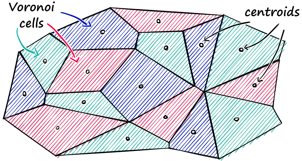
2.Partitioning Index (faiss.IndexIVFFlat) –
Partition Index uses Voronoi cells to partition vectors. It checks the distance between the query vector and each cell’s centroid, limiting the search to vectors within the nearest centroid cell. The number of centroids for the final search can be chosen using the option index. Probe.
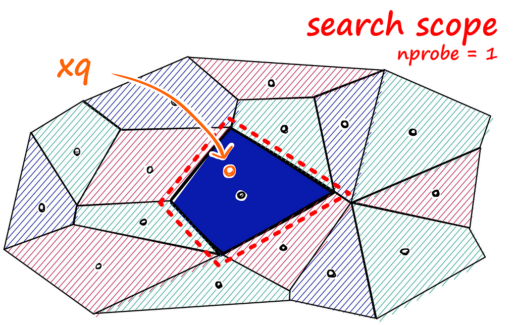
xq is the query vector and nearest centroid is present in the highlighted blue cell. We have chosen nprobe=1 so only one cell is selected.
From observation on different use cases, we noticed that with a larger number of centroids, the search is faster, but less accurate compared to an exhaustive (Flat L2) search.
Pros:
Redundant search against all vectors is removed since we have limited the scope to the nearest centroid.
Cons:
There might be closest point in another Voronoi cell this is the factor which we compensate for speed.
3.Product Quantization (faiss.IndexIVFPQ) –
In product quantization, the vector dimension is reduced to chunks and clustering is performed to obtain a centroid id which acts as a look up book for vectors. Finally, when query-vector comes it is divided into sub-vector and a lookup book is used to identify the distance of each sub-vector with all the cluster centroids.
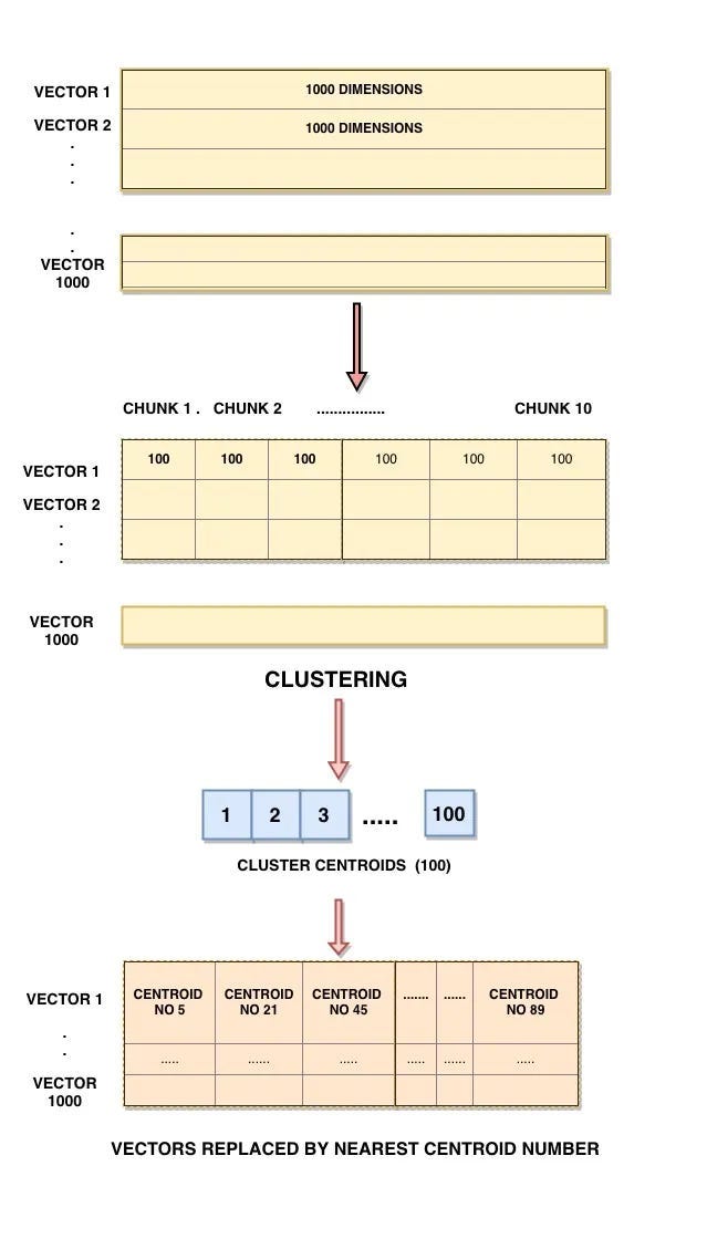
Image Reference from blog (top to bottom flow)
Pros:
It is a great way to compress a dataset. It is 18 to 20 times faster than other indexes.
Cons:
Results vary from both partitioning index and flat index. If speed is the major concern, then PQ is considered.
We notice that to obtain most accurate results its preferable to use Exhaustive Search (Index Flat L2).
Faiss allows merging of different indexes using index factory, offering flexibility and enhanced memory efficiency in combining various approaches.
index = faiss.index_factory(128, “IVF10000_HNSW32, PQ16”)
# combining HNSW with PQ (it is 15 times more memory efficient than HNSW alone as per experiments).
Now that we have gained insights into these Faiss indexes, let us further explore their practical applications using real-world data and analyse the observations derived from their implementation.
Implementing the Semantic Search Approach for Classification:
1.Data Cleaning:
- Start by cleaning the data through essential pre-processing steps, including tokenization, punctuation removal, lowercase conversion, and elimination of stop words.
2.Embedding Generation:
- Obtain embeddings for the text data using any approach, such as TF-IDF, Glove, or sentence transformer embeddings (we utilized MiniLM-l6-V2).
3.Integration with Faiss Library:
- Transfer these embeddings to the Faiss library after selecting the appropriate index type (flat index, partitioning index, or product quantization).
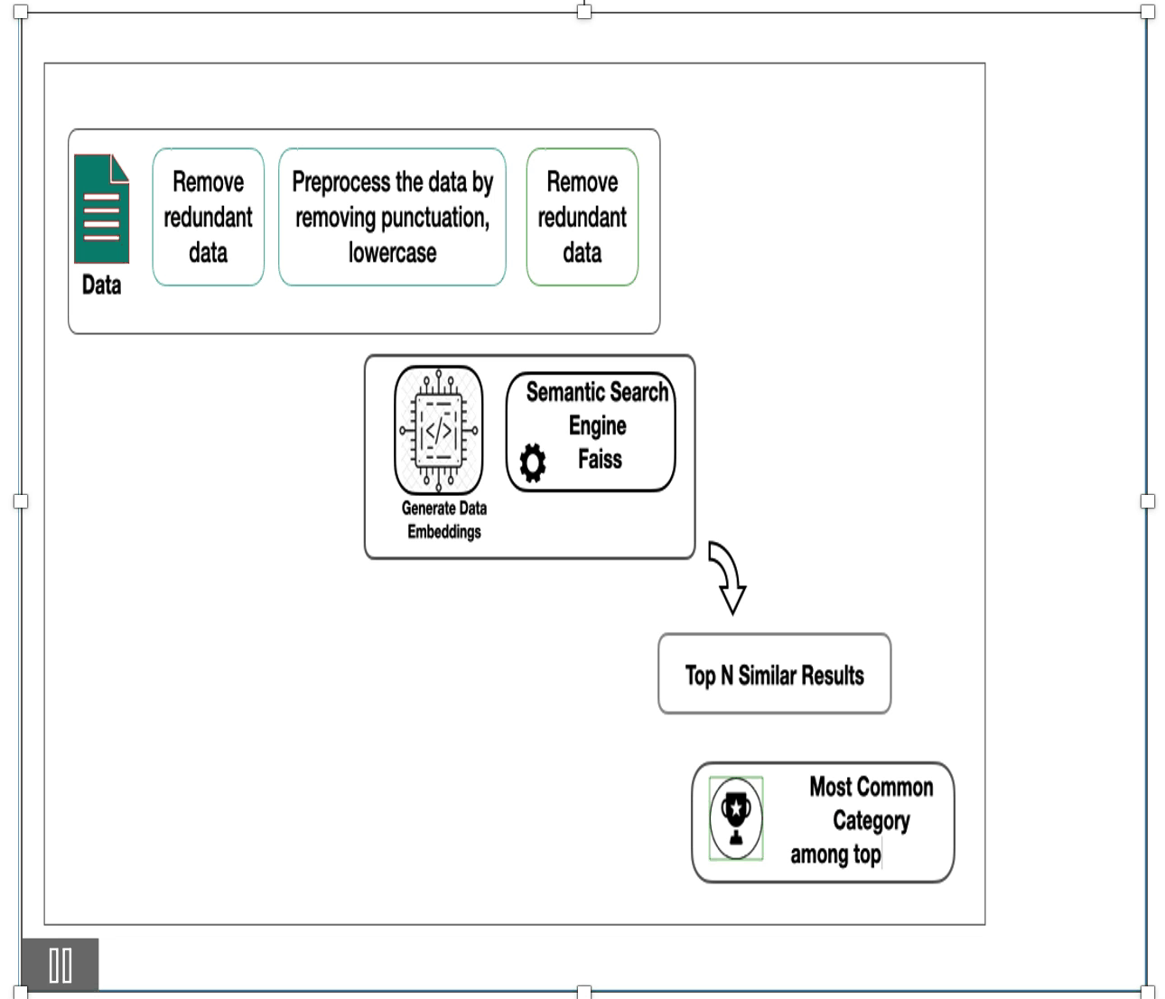
4.Query Embedding Retrieval:
- Retrieve the embedding for a given input test query using the same model chosen in step 2.
5.Faiss Index Search:
- Utilize Faiss index to search for similar sentences. This process returns the top N similar sentences for the input query along with their scores.
6.Category Retrieval:
- Obtain the categories of the returned top N similar sentences using a mapping dictionary that correlates sentences to categories.
7.Classification Decision:
- Determine the final output class by either selecting the maximum category count from the top N or applying other statistical ranking methods for the given input.
Original Data:
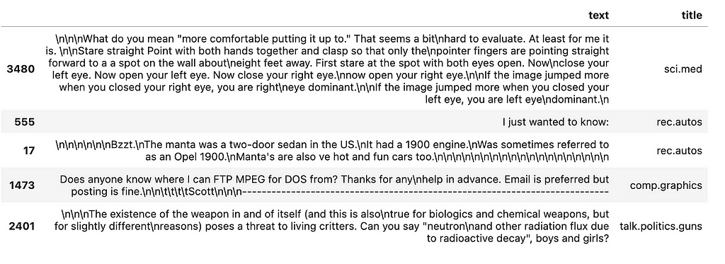
dataset
- Basic cleaning steps has been followed as mentioned in the step1 after removing redundant data.
def clean(text):
    text=text.lower()
    url_removed=re.sub(r'https\S+','',text,flags=re.MULTILINE)
    text=re.sub("[^a-zA-Z]"," ",url_removed)
    text=re.sub("\.+"," ",text)
    text=[word for word in text if word not in string.punctuation]
    text="".join(text).strip()
    text=re.sub("\s\s+", " ", text)
    return "".join(text).strip()
selected["cleaned_data"]=selected["text"].apply(lambda x:clean(x) if x!=None else x)
Choosing embeddings is the main key point for obtaining good results. Utilising all-minilm-l6-v2 for this usecase
model=SentenceTransformer('sentence-transformers/all-MiniLM-L6-v2')
def get_embeddings(model, sentences: List[str], parallel: bool = True):
    start = time.time()
    if parallel:
        # Start the multi-process pool on all cores
        os.environ["TOKENIZERS_PARALLELISM"] = "false"
        pool = model.start_multi_process_pool(target_devices=["cpu"] * 5)
        embeddings = model.encode_multi_process(sentences, pool, batch_size=16)
        model.stop_multi_process_pool(pool)
    else:
        os.environ["TOKENIZERS_PARALLELISM"] = "true"
        embeddings = model.encode(
            sentences,
            batch_size=32,
            show_progress_bar=True,
            convert_to_tensor=True,
        )
    print(f"Time taken to encode {len(sentences)} items: {round(time.time() - start, 2)}")
    return embeddings.detach().numpy()
Choosing the index type followed by creating and saving is next step
# we have used flat Index and with Inner product here but another experiment in repo has partition index
def create_index(mappings,samples):
    index = faiss.IndexIDMap(faiss.IndexFlatIP(samples.shape[1]))
    faiss.normalize_L2(samples)  # normalise the embedding
    #index.train(samples)
    index.add_with_ids(samples,np.array(list(mappings.keys())))
    save_index(index)
create_index(mappings=mappings,samples=samples)
Last step is to read the index, search the query inside the index and obtain top N results and predicting for user query given mapping of categories
#read the index
index = faiss.read_index("./data/news_train_index")
# embeddings for query
def predict_embeddings(query):
    query_embedding=model.encode(query)
    query_embedding=np.asarray([query_embedding],dtype="float32")
    return query_embedding
#predict for given query
def predict(query,mappings):
    cleaned_query= clean(query)
    query_embedding=predict_embeddings(cleaned_query)
    faiss.normalize_L2(query_embedding)
    D, I = index.search(query_embedding, 10) # d is the distance and I is the index number
    D=[np.unique(D)]
    I=[np.unique(I)]
    res_df=[]
    for values in I:
        for val in D:
            details= {'cleaned_text':list(train.iloc[values]["cleaned_data"]),
            'category':list(train.iloc[values]["title"]),
            'score':list(val)
            }
            res_df.append(details)
    return res_df
Example 1:
res=predict("glycemic index",mappings=mappings)
# score is actually distance so lower is better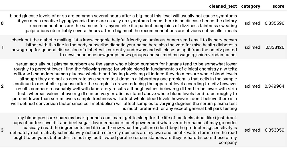
def most_frequent(result):
    top2 = Counter(result)
    return top2.most_common(1)
Results of top 5 similar sentences belong to the category sci.med and from above function the most common is sci.med. Hence the final class we considered is sci.med.
Example 2
res=predict("cad tools utilises graphics card the quality of image depends on the quality of graphics card.",mappings=mappings)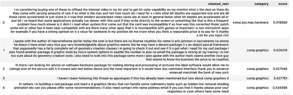
The above example returns top 5 from two categories but most common is graphics class. Hence final class for the query is graphics.
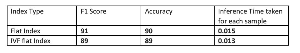
Comparison of results with flat index and ivfflat index:
More details about entire logic for different indexes mentioned above are available in the GitHub repository — refer to readme for installation steps.
Conclusion:
Faiss is known for its user-friendly nature, making installation and usage hassle-free. The library is compatible with both GPU and CPU, adding to its versatility. It boasts exceptional speed, excelling in both index creation and searching. It is important to be aware that adding new data to an existing index is not currently supported. Instead, creating a new index is required, but the process is quick, so there is no need for significant concern about time consumption.
References:
https://github.com/Harika-3196/classification-using-faiss-semantic-search-index
https://www.pinecone.io/learn/faiss-tutorial/
https://github.com/facebookresearch/faiss/wiki/Getting-started
Tags:
Semantic Search Classification Faiss Scaling
Transforming Text Classification with Semantic Search Techniques — Faiss was originally published in Walmart Global Tech Blog on Medium, where people are continuing the conversation by highlighting and responding to this story.