
Tags: #DataScience #CausalInference #DifferenceinDifference #Matching #MatchedDiD #PropensityScoreMatching
E-commerce businesses often introduce treatments (decisions) for their customers and want to measure the impact of those treatments on metrics of interest. For example, an e-commerce subscription business often faces the challenge of determining whether changes in member benefits result in increased spending or retention. The most reliable way to assess the causal impact of such changes is through randomized experiments via A/B tests. In some cases, conducting an A/B test is not feasible due to a lack of control group, resource limitations, or strategic business decisions.
In such situations, quasi-experimental techniques like difference-in-difference, regression discontinuity, and synthetic controls can be used to estimate the causal impact of the treatment. However, these techniques are susceptible to confounding effects from other variables. For instance, when introducing a new benefit in an e-commerce subscription, factors such as a member’s tenure, existing engagement with the platform, pricing, or promotional campaigns may affect basket size, spending, or retention, and not necessarily the benefit itself. This means that the difference in the outcome metric may be caused by a confounding variable like the level of motivation rather than the treatment status.
To address the limitations of traditional quasi-experiment techniques, we propose a framework called Adopter Analysis. It is comprised of three techniques: defining an adopter, propensity score matching and difference-in-difference (DiD). In the following sections, we will discuss each technique in detail.
Defining an Adopter
To begin the analysis, we define an adopter as a user who has utilized a benefit at least once. For certain benefits, such as an item price discount that can be redeemed in the next purchase, we may consider two purchase cycles as the adoption threshold. This will help us to create treatment and control groups, with the treatment group comprising adopters and the control group comprising non-adopters. In Python, we can define adopters using the following method:
data[‘adopter’] = 1 if data.benefit_usage_count >= 1 else 0
Propensity Score Matching
Selection bias often occurs in observational studies, where participants are not selected randomly, and researchers choose the subjects. Propensity score matching is a technique that aims to minimize selection bias by creating comparison groups with similar observed characteristics. This is done by selecting a control group with characteristics similar to the treatment group and then comparing their outcomes. Propensity score matching is based on the probability of treatment assignment, given observed baseline covariates, such as demographics, prior engagement with the platform, and tenure. By doing this, we can create comparable treatment and control groups. In our example, we calculated the propensity of a member to be exposed to a subscription benefit in the pre-treatment period. We would match two members from the treatment and control groups, respectively, based on their propensity scores, which should be within a specified threshold.
logit (Pr(Treatment = 1|Covariates)) = β0 + β1X1 + β2X2 + … + βkXk
where:
logit (Pr(Treatment = 1 | Covariates)) is the log odds of the member seeing the subscription benefit
Pr(Treatment = 1 | Covariates) is the probability of the member seeing the subscription benefit
β0 is the intercept term.
β1, β2, …, βk are the coefficients of the independent variables or co-variates.
x1, x2, …, xk are the independent variables.
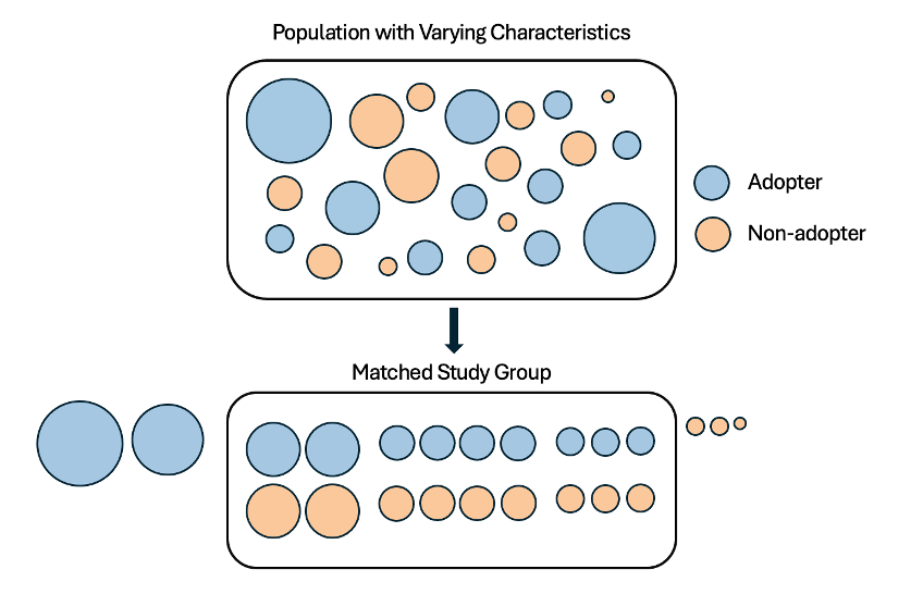 Result schematic of propensity score matching.
We can evaluate the matches by examining the propensity scores plot before matching and by comparing the means of the original and matched data. Miroglio has also explained how to evaluate matches at the continuous and categorical variable levels. Essentially, we test whether the data is “balanced” across our co-variates. For categorical variables, we look at plots comparing the proportional differences between test and control before and after matching. For continuous variables, we look at Empirical Cumulative Distribution Functions (ECDF) for our test and control groups before and after matching.
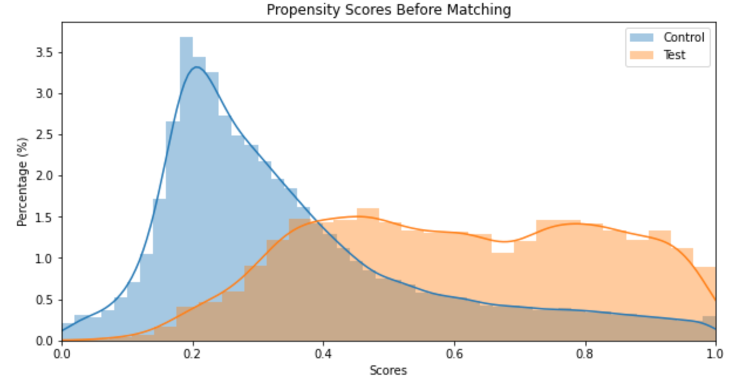 test vs. control or adopter / non-adopter propensity distributions before matching
As we can see in the chart, the test and control groups (adopters and non-adopters) are already separable before matching, which means matching is required to account for confounding variables and get an accurate estimate of the true treatment effect.
Sometimes, however, matching before applying DiD can sometimes introduce bias in the estimates instead of reducing bias by undermining the second difference in the DiD via a regression-to-the-mean effect. Dae Woong Ham and Luke Miratrix explain in detail and provide a heuristic guideline to best reduce bias. Therefore, we should evaluate the need for matching on case-by-case basis and use appropriate matching methods to get desired unbiased causal estimates.
Difference-in-Difference
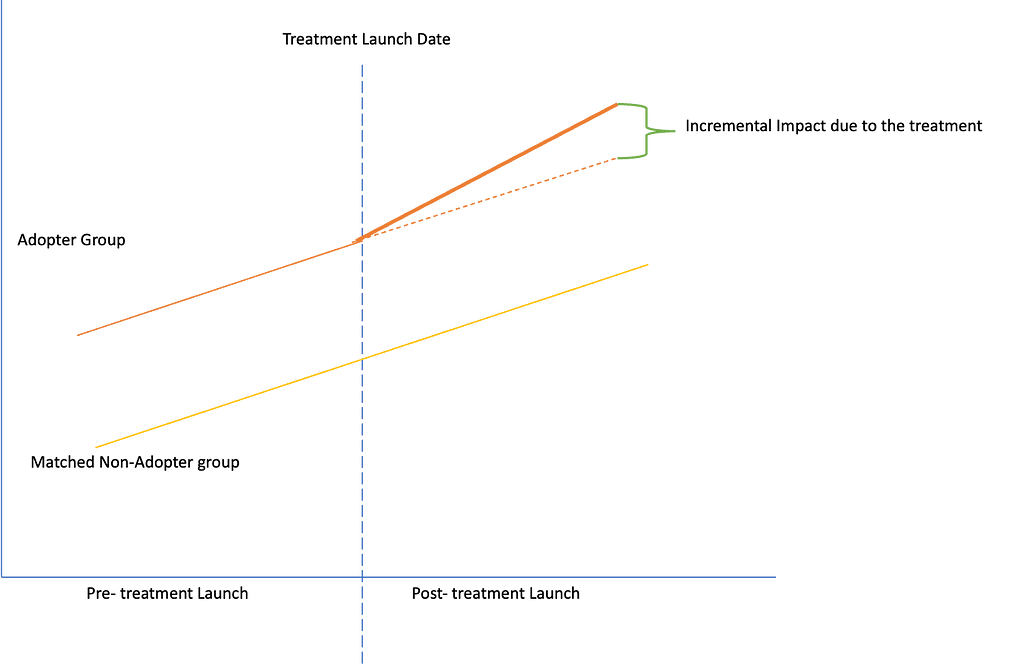
Once we have matched the treatment and control groups on observed characteristics, we can then use difference-in-difference to estimate causal impact. By using matching before applying DiD, we take care of the assumption that treatment group and control group must follow the same trend in the pre-period. In the price discount example, we would simply compare changes in spend, basket size and retention over time in the treatment group to changes in control group. If there is a significant difference in the changes between the two groups, this would suggest that the intervention had a causal impact on spend and retention.
Here is how we would do it in Python for the output metric Spend:
Aggregating the matched pairs from the treatment and control groups, we calculate the difference-in-difference estimate, i.e., the Average Treatment Effect (ATE):
Impact(Y) = (Yt_post — Yt_pre) — (Yc_post — Yc_pre)
where:
Yt_post = avg treatment_post
Yt_pre = avg treatment_pre
Yc_post = avg control_post
Yc_pre = avg control_pre
Thus, the combination of defining adopters, propensity score matching, and difference-in-difference can make more robust inferences than the individual techniques when randomization is not feasible. To demonstrate this further, we compared the Average Treatment Effects using canonical Difference-in-Difference vs. using Adopter Analysis. Here are the results:
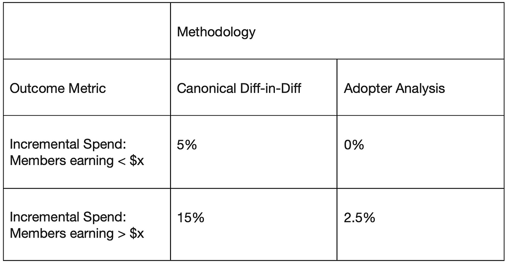
Here, we see that canonical difference-in-difference tends to over-estimate the impact of a treatment on outcome metrics. By accounting for both selection bias and unobserved confounding, the Adopter Analysis approach can help obtain more accurate estimates of the causal impact and make more informed decisions about a benefits’ impact on member metrics and other interventions in the world of retail and e-commerce.
Acknowledgments:
Thank you to Srujana Kaddervamuth for the problem statement of the research, Sambhav Gupta for ideation and brainstorming on this approach, Pratika Deshmukh for helping with the data querying and aggregation. Katherine Wang, Haley Singleton, and Lindsey Soma for approach feedback and brainstorming. Thank you Ravishankar Balasubramanian, Jonathan Sidhu, Saigopal Thota and Rohan Nadgir for support and guidance.
References:
[1] Ben Miroglio, “Introducing the pymatch Python Package,” Medium, Dec 4, 2017, Available: https://medium.com/@bmiroglio/introducing-the-pymatch-package-6a8c020e2009 [Accessed May[A1] 1, 2023]
[2] Dae Woong Ham and Luke Miratrix, “Benefits and costs of matching prior to a Difference in Differences analysis when parallel trends does not hold,” Arxiv, 17 May 2022 , Available: https://arxiv.org/abs/2205.08644 [Accessed Feb 5, 2024]
How to Determine Causal Effects when A/B Tests are Infeasible through Adopter Analysis was originally published in Walmart Global Tech Blog on Medium, where people are continuing the conversation by highlighting and responding to this story.