 Photo from Unsplash
Why Causal Analysis?
Causal analysis enables us to understand the underlying causes and relationships between interventions (treatments), variables, and outcomes. It provides insights on the cause-and-effect relationships between variables or events, helping business to understand the factors that influence the outcomes. Based on this understanding, more informed and effective strategic decisions can be implemented, predicting the potential impacts and consequences. Now, let’s understand why Causal Analysis is important:
a. Causation is not Correlation: Correlation is defined as how closely the variables are related or how they tend to change together. However, just because two variables are correlated does not necessarily mean that one variable is causing the other to change.
For example, the number of firefighters and number of fire breakouts can have a high correlation, but number of firefighters are not causing more fire breakout event. It’s the opposite that more fire breakouts might cause the department to need more firefighters.
To establish causality between two variables, several conditions need to be met:
- Temporal relationship: The cause must occur before the effect.
- Consistent Association between variables: The cause and effect should consistently occur together.
- Plausible Explanation: How the cause leads to the effect. This should be supported by existing knowledge and theories.
b. Alternative to A/B testing: Causal analysis and A/B testing are two different methods to understand the causal impact. While both methods have their advantages, causal analysis is often considered better than A/B testing for several reasons:
- Causal analysis allows identification and control of confounders to isolate the impact of the treatment. Whereas in A/B testing, it is difficult to control for confounders and eventually it leads to inaccurate interpretations of the impact measure.
- Moreover, A/B testing often requires significant resources and time to implement and analyze compared to Causal analysis.
How it can be Used?
Causal Analysis helps to measure the impact of the treatment and attribute the impact to different factors. These two are use-case agnostic and can be used in various fields, including policy evaluation, retail, marketing, healthcare, finance domain.
Causal Impact: It helps to quantify the degree of influence on the outcome due to the presence of an intervention vs. absence of the intervention, while other variables remain same.
Causal Attribution: It helps to identify the specific factors or variables that influence the outcome based on various data.
Basic Concepts for Causal
Let’s understand few basic concepts on causal analysis before moving forward:
a) Markov-Equivalence and d-separation: d-separation is a criterion for deciding whether a set X of variables is independent of another set Y, given a third set Z. For three disjoint sets of variables X, Y, and Z; X is d-separated from Y conditional on Z if and only if all paths between any member of X and any member of Y are blocked by Z. For more details, go through the link.
Graphs that have the same d-separation properties are termed as ‘Markov equivalent’ and imply the same conditional independence relations. A collection of all directed acyclic graphs (DAG) that are Markov equivalent is a ‘Markov Equivalence Class’ (MEC). d-separation can be generalized to directed acyclic graphs (DAG) when:
(i) There are no cycles present in the graph i.e. acyclic in nature
(ii) The graph is directed i.e. the edges have specific direction
b) Directed Acyclic Graph (DAG): DAG is a conceptual representation of potential causal relationships among the variables by a graph. These relationships are established by joining the nodes (variables) along with directed edges (arrows). An arrow from one variable to another indicates that the former variable causally influences the later one. The most important feature of DAG is its acyclic nature, which ensures that there are no feedback loops, where a variable directly or indirectly causes itself.
DAG helps to identify the Counterfactuals and Instrumental variables, which is important to structure the problem for causal analysis.
C) Confounders: Confounders are the variables that impact the treatment and outcome variable. Confounders can lead to spurious associations between the treatment and the outcome, making it difficult to determine the true causal relationship by introducing bias.
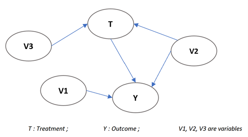 Image by Author
In the above graph, V2 is the confounder as it impacts both Treatment and Outcome.
d) Instrumental variables (IV): Instrumental variables are directly related to the treatment variable (T) but not directly with the outcome variable (Y). It impacts the outcome variable only through treatment. By using an instrumental variable, we can isolate the causal effect of treatment on outcome by removing the bias due unobserved confounding factors.
In the above graph, V3 is the instrumental variable as it impacts the treatment but does not directly affect the outcome variable.
e) Counterfactual: Counterfactual is a concept of alternate reality to compare what has happened (observed outcome) vs what would have happened if the treatment was not applied, or different treatment was applied (counterfactual outcome). It helps to estimate the causal effect of the treatment by comparing the observed outcome with the counterfactual outcome.
Say, we want to measure the impact of a marketing event on sales.
Actual: What has happened on sales due to the new Marketing event
Counterfactual: What would have happened if the new Marketing event wasn’t introduced
— Then we try to measure the difference as an impact between these two scenarios.
Different Methods for Causal Discovery
There are different methods to perform causal discovery and construct DAG. Few commonly used algorithms for DAG are:
a) Peter-Clark (PC) Algorithm: This is a constraint-based causal discovery method which is consistent under independent and identically distributed (i.i.d) sampling assuming no latent confounders. It is based on topological sorting (Partially ordered set) which helps to find an ordering of the vertices and thus reachability relation in a DAG.
Under the causal Markov condition, PC assumes there is no latent confounder, and two variables are directly causally related if there is no subset of the remaining variables conditioning on which they are independent.
Illustration of how the PC algorithm works:
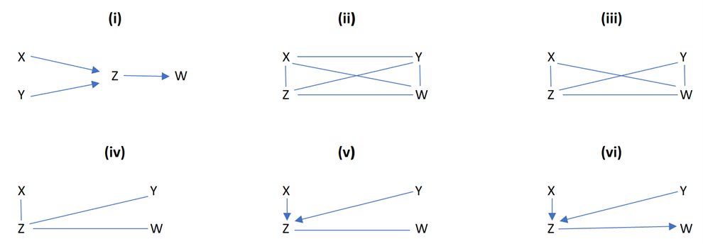 Image by Author
(i) Original true causal graph: By d-separation, this structure implies that X is independent of Y, written X ⫫ Y, and that X and Y are each independent of W conditional on Z, written {X, Y} ⫫ W|Z
(ii) PC starts with a fully connected undirected graph.
(iii) The X − Y edge is removed because X ⫫ Y. (unconditionally independent)
(iv) The X − W and Y − W edges are removed because X ⫫ W | Z and Y ⫫ W | Z. (conditionally independent)
- This can be extended to multiple variables like X ⫫ W | {Z1, Z2, …, Zn}
(v) Finding V-structures (triple of variables). Here, Z was not conditioned on in eliminating the X−Y edge, so orient X−Z−Y as X → Z ← Y
(vi) Orientation propagation: For each triple of variables such that Y → Z−W, and Y and W are not adjacent, orient the edge Z−W as Z → W.
If the cyclicity is found in the graph, the algorithm will not terminate or produce an incorrect ordering. It also allows data sets with missing values.
b) Fast Causal Inference (FCI) Algorithm: This is a generalized version of PC algorithm which tolerates and sometimes discovers unknown confounding variables. Its results have been shown to be asymptotically correct even in the presence of confounders.
c) Greedy Equivalence Search (GES) Algorithm: This is a score-based (BIC or generalized) causal discovery method. By iteratively adding or removing edges through greedy algorithm, it helps to create the DAG.
Illustration of how the GES algorithm works:
(i) This method starts with an empty graph unlike PC or FCI.
(ii) At each step, the decision is made whether to add a directed edge to the graph will increase the fit measured by some quasi-Bayesian score such as BIC, or even by the Z score of a statistical hypothesis test.
(iii) The resulting model is then mapped to the corresponding Markov equivalence class, and the procedure continued.
(iv) When the score can no longer be improved, it checks edge by edge, which edge removal (if any), will most improve the score, until no further edges can thus be removed.
d) Linear Non-Gaussian Acyclic Models (LiNGAM) based Methods: It is a family of methods that assumes the relationships between variables to be linear and non-Gaussian.
The linear causal model in the two-variable case can be written as: Y= bX + ε, where ε ⫫ X.
Now, assume Y is generated from X in a linear form, i.e., Y = X+ε, where ε ⫫ X. Now let’s consider 2 scenarios:
Regression of Y given X: Plot two variables X and Y, and X and regression residual (ε).
Regression of X given Y: Plot two variables X and Y, and Y and regression residual (ε).
Also, consider 3 cases each under above 2 scenarios, and those are X and ε follows (i) Gaussian distribution (ii) Uniform distribution (iii) Any other non-gaussian distribution.
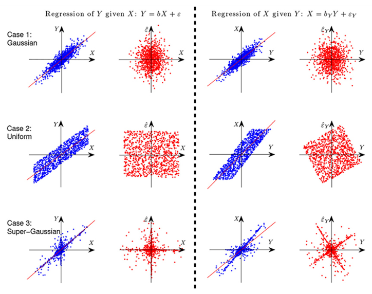
From the above graph, it is observed that for last 2 non-gaussian cases, regression of X given Y indicates that the ε is not independent from the predictor anymore, although they are uncorrelated by construction of regression.
In short, if at least one of X and ε is non-Gaussian, then the causal direction is identifiable (Darmois-Skitovich theorem). There are different types of LiNGAM-based methods (e.g., ICA-LiNGAM, Direct-LiNGAM, VAR-LiNGAM). For More details, go through the link.
Each method has its own strengths and limitations, and the choice of method depends on the specific data and problem statement in hand. Apart from these algorithms, there are a variety of algorithms available. In python, CausalLearn library helps to implement these algorithms and identify the DAG. For more details, have a look at this link.
Different Methods for Causal Estimate
a) Difference-in-Difference (DiD): It is a quasi-experimental approach that compares the changes between pre and post time and between a population enrolled in the treatment group and a population that is in the control group. As we are measuring the differences in two cases, hence the name difference-in-difference.
The impact of DiD is measure as:
(Treatment_Post —Treatment_Pre) — (Control_Post — Control_Pre)
Mathematically, the equation can be written as:
y= α+ β1 diff_1 + β2* diff_2 + γ*(diff_1 * diff_2) + ∈
where,
diff_1: Whether the observation is in the treatment group (1) or the control group (0)
diff_2: Whether the observation is before the treatment introduced (0) or after the treatment introduced (1)
diff_1 * diff_2: Interaction term
Matching algorithms can also be used to define the control group, by balancing the distribution of confounding variables in the treatment and control groups. This will help to reduce bias. We match each entity from the treatment group with one or more entities from the control group that have similar values of the confounding variables. This pseudo-randomized experiment helps to measure the impact of the treatment more accurately. There are different matching algorithms such as propensity score matching, nearest neighbor matching etc.
b) Bayesian Network: It is a probabilistic graphical model that represents a set of variables and their conditional dependencies via a directed acyclic graph (DAG). The mathematical representation of a Bayesian network is a joint distribution of all variables.
For causal inference, we use do-calculus introduced by Judea Pearl. The fundamental equation of do-calculus for a variable X do(X=x) in a Bayesian network is:
P(Y/do(X=x) = ⅀ P(Y | X=x,Z=z) * P(Z)
where, Z is a set of variables that satisfies certain conditions called backdoor criteria. This allows us to compute the causal effect of X on Y.
c) DoWhy and EconML: This is a python-based library, focuses on causal inference and causal reasoning. This includes four main steps:
- Defining causal models (using DAG)
- Identifying causal effects and return target estimands
- Estimating the identified estimands using statistical methods (like Propensity Score Based Methods, Instrumental Variable Methods, Double Machine Learning, Front Door Adjuster etc.)
- Refuting the estimated causal effects via robustness checks (like random common cause, placebo treatment refuter, data subset refuter etc.)
d) CausalImpact: CausalImpact helps to estimate how the time series would have evolved after the intervention if the intervention had not occurred. It uses Bayesian structural time-series models to measure the impact. This approach is useful where a randomized experiment is not feasible and especially in small sample scenarios.
It provides posterior distributions along with point estimates of causal effect. It assumes that there are no confounders that simultaneously affect the control and target at the time of the intervention.
In summary, the choice of these algorithms depends on the specific requirements of the problem statement, including the nature of your data, the complexity of your causal question, and your computational resources.
Usually as standard practice, Difference-in-Difference is a common method, but this is mostly useful when information on both pre- and post-treatment period is available. Otherwise, Bayesian Network or/and DoWhy-EconML helps to estimate the impact using counterfactual, though Bayesian Network depends on probabilistic relationships among the variables.
But all these 3 algorithms are not able to include the time series impact. We need to measure the impact for every time point separately to check the trend of the impact. Whereas CausalImpact helps to measure the causal impact of intervention over time.
Python Libraries for Causal Discovery and Causal Impact
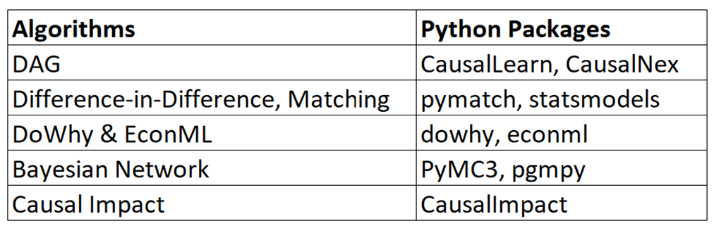 Image by Author
Measure the Impact of the Treatment
The impact or effect of the treatment/intervention can be measured at the overall population, treatment group and subgroup levels.
a) Average treatment effect (ATE): ATE measures the average difference in outcomes between a treated group and a control group. ATE, measured at overall population level, is defined as:
ATE = E[Y(T = 1) — Y(T = 0)]
where, T : treatment
Y(T = 1) : potential treated outcomes for entire population
and Y(T = 0) : potential control outcomes for entire population
b) Average treatment effect on treated (ATT): ATT measures the average difference in outcomes between those who received the treatment and those who did not within the treated group. ATT, measured at treated group level, is defined as:
ATT = E[Y(T = 1)|T = 1] — E[Y(T = 0)|T = 1]
where, Y(T = 1)|T = 1 : potential treated outcomes of the treated group
and Y(T = 0)|T = 1 : potential control outcomes of the treated group
c) Average treatment effect on control (ATC): ATC measures the average difference in outcomes between those who received the treatment and those who did not within the control group. ATC, measured at control group level, is defined as:
ATC = E[Y(T = 1)|T = 0] — E[Y(T = 0)|T = 0]
where, Y(T = 1)|T = 0: potential treated outcomes of the control group
and Y(T = 0)|T = 0: potential control outcomes of the control group
d) Conditional average treatment effect (CATE): CATE measures the average difference in outcomes between a treated group and a control group within a subgroup. It is also known as the heterogeneous treatment effect as treatment effect varies across different subgroups. CATE, measured at subgroup level, is defined as:
CATE = E[Y(T = 1)|X = x] — E[Y(T = 0)|X = x]
where Y(T = 1)|X = x : potential treated outcomes of the treated subgroup with X = x
and Y(T = 0)|X=x : potential control outcomes of the treated subgroup with X = x.
Now let’s understand which metrics we should consider based on use cases:
ATE: should an intervention be offered to everyone who is eligible?
ATT: should an intervention currently being offered, should continue or withheld?
ATC: should an intervention be extended to people who don’t currently receive it?
CATE: should an intervention be offered to everyone who is eligible within a subgroup?
Here, we have only focused on binary treatment, but it can easily be extended for multiple treatment.
Industry use Cases
Causal Inference has a vast use case across industries for policy or strategy implementation standpoint as it aids decision-making by understanding cause-and-effect relationships. Businesses use the causal analysis for informed decision-making processes. By understanding the cause-effect relationships between different business variables, companies can make informed decisions about strategy and operations. Few examples which can be supported through Causal to improve/help Business are:
a. Medical Evaluation: Causal analysis is vastly used to diagnose diseases by analyzing medical history, symptoms or/and various test results. This helps in predicting the possible illness that a patient might have. Also, Causal analysis helps to measure the impact of a newly introduced medicine.
b. Policy Evaluation: Causal analysis is used to understand the impact of various policies on different outcomes. This helps in decisions making about policy implementation and modification.
c. Retail Industry: Causal Analysis helps to measure the impact of any promotional event on sales amount or to measure the impact of marketing strategies on Ads and Click through rate.
d. Traffic Management: In traffic management, causal analysis is used to understand the impact of various factors on traffic congestion. This can help in developing strategies to reduce congestion and improve traffic flow.
Fundamentals of Causal Discovery and Causal Impact Analysis was originally published in Walmart Global Tech Blog on Medium, where people are continuing the conversation by highlighting and responding to this story.
Article Link: Fundamentals of Causal Discovery and Causal Impact Analysis | by Prasun Biswas | Walmart Global Tech Blog | Mar, 2024 | Medium