Automated Input Data Distribution In a Multinode Workflow
Authors: Sandesh Balakrishna | Mohsin Kaleem
Designing a ML workflow at scale requires multiple considerations — important being memory, Time To Run (TTR), Cost To Run (CTR). Workflows must be designed to maintain a balance of these metrics. There may be use cases where a single node workflow might not be sufficient either in memory or run time SLA (Service Level Agreements) adherence given that each node of a workflow will have a capacity constraint: Memory/CPU in case of Python or number of executors that the node may use in case of Py-spark. Given these constraints the opportunity for parallelism is also limited. Code modularization is another factor that contributes to the above metrics along with providing other benefits. This blog presents a use case where code modularization and workflow parallelization (aka flows) came together to improve the performance of a Prophet Time series forecasting algorithm scaled across hundreds of categories and 5 different countries. We also present a code package for automated input data distribution across the different flows of a workflow.
An example is shown below where a time series forecasting algorithm using prophet on Py-spark had to run for around 150 categories. A single node workflow design presented the following challenges:
1. Resource assignment/utilisation may not be optimal while using distributed computing frameworks like spark resulting in longer times. A data preparation module requires resources (CPU and memory) different from a ML algorithm module.
2. Difficult to monitor at what stage the flow is at any point in time unless extensive in-code logging is enabled
3. Restarting from the point of failure is difficult leading to longer run time for a module
 Monolithic Design
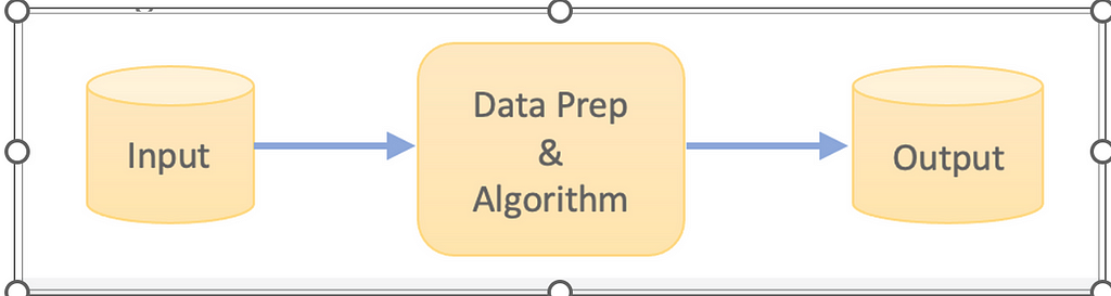
The alternative is to modularize the code into separate units for data prep and algorithm. Groups of categories aka flows were also created where each flow contains all the steps (data prep, algorithm, post processing etc) required for an end-end run and runs parallelly independent of another. A combiner at the end unions the output of every flow to be exported to the downstream layers. Every node in the below design accesses the same code base which improves maintainability. In the below diagram, Data-Prep-A to Data-Prep-F run in parallel and access a common data preparation run file while Algorithm-A to Algorithm-F running in parallel access a common ML run file.
 Modular Design
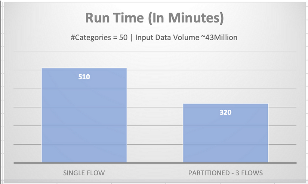
The below chart captures the run time boost gained by the parallelization in one of our projects:
An experiment with 50 categories and input record count of ~43 million rows was run with and without modularisation. The categories were passed through a single flow resulting in a run time of 8.5 hours. The categories were also split and distributed between 3 flows resulting in a run time of 5 hours 20 minutes which is 1.59 times faster.
 Execution Time Monolithic Design Vs Modular
To ensure a balanced run, the data volume must be uniformly distributed across each of the flows. Distributed frameworks like Py-spark also work best when the amount of data provided to executors is similar. Hence the mapping of categories to the flows requires a balancing act! Manually generating the flow-category mapping is quite tedious when we scale to different markets or geographies. The data distribution also keeps changing in a dynamic production environment. Wouldn’t it be great if the flow-category mapping is generated automatically?
The code base below explains a way to automatically create this mapping while balancing the distribution metric for each flow (Metric could be total number of records in each flow)
Code Snippet and explanation:
We can reframe our problem statement to an algorithmic task — “Given an array with non-negative elements, split it into K (Number of flows) sub-arrays such that the maximum sum of all sub-arrays is minimum.”
Example — Input: Array [] = {1, 2, 3, 4}, K = 3
1. best case:
Optimal bucket size: 4 [i.e. at max we can have a total of 4 records in a bucket]
Optimal split: {1, 2}, {3}, {4}, here the maximum sum of all subarrays is 4 [which in this case is minimum] given k=3
2. non-optimal case:
bucket size: 5
bucket splits: {1}, {2,3}, {4} -> Over here maximum sum of all subarrays is 5 [non-optimal case as there is a possibility of even lower value]
A Naive approach:
1. A naive approach would be to find all possibilities of k such sub-arrays using backtracking.
2. Find the sum of the sub-array and take the case where the sum of those k sub-arrays is minimum.
This approach has a very high time complexity and would be extremely slow if the array size is large.
An Efficient Approach:
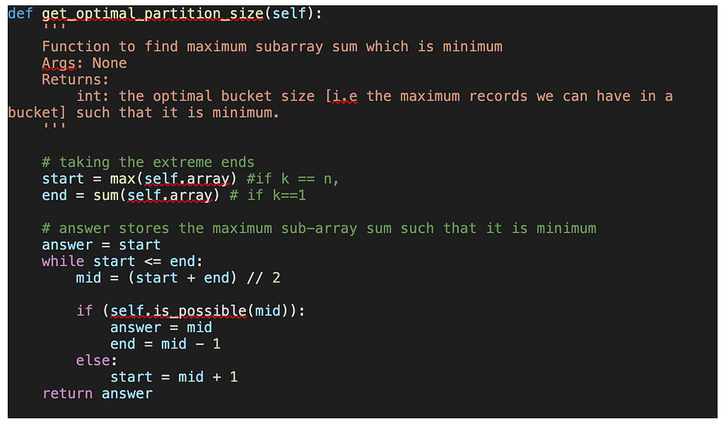
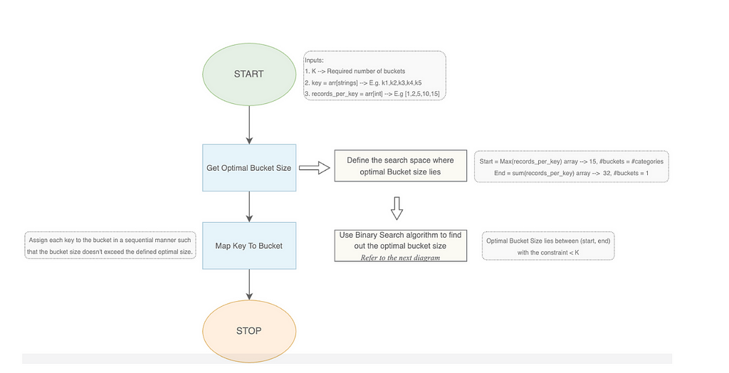
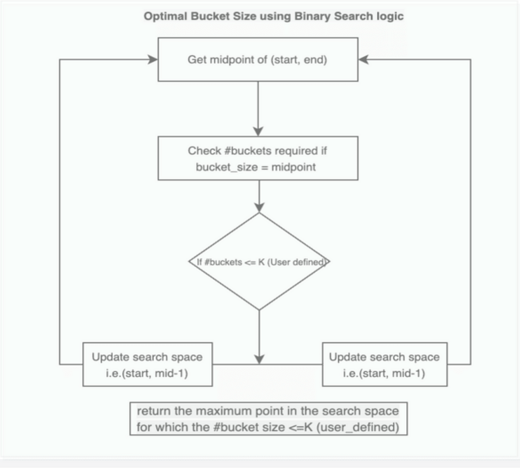
[Step — 1] The idea is to use a binary search algorithm to find the optimal bucket size [i.e. the maximum records we can have in a bucket] such that it is minimum. The range of the search is defined by the lowest and highest possible values where:
The lowest value would be the max element of the array, when the number of buckets is equal to the size of the array i.e. k=n. Here we can allot the max element to one bucket and divide the other sections such that the sum of those sub-array is less than or equal to max.
The highest value would be the sum of all the elements in the array and this happens when we allot all the records of the array to one bucket i.e. k=1
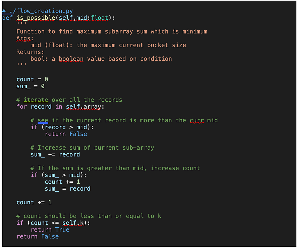
Then in each iteration, we try to get the minimum possible value of mid which satisfies the condition:
Number of buckets counts we get using the mid value as our bucket size should be less than the actual k, and it should cover all the array’s element
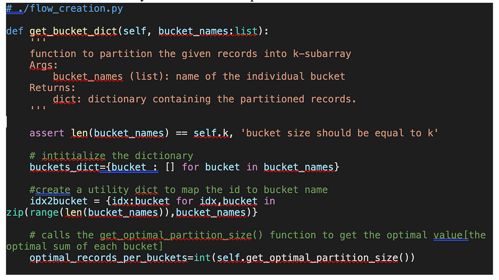
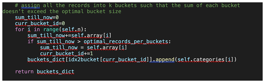
[Step — 2] Then partition the array records into k buckets once we get the optimal size of the bucket such that the distribution metric [i.e. sum of the records of each bucket] is similar. Then returns the dictionary which contains the partitioned records.
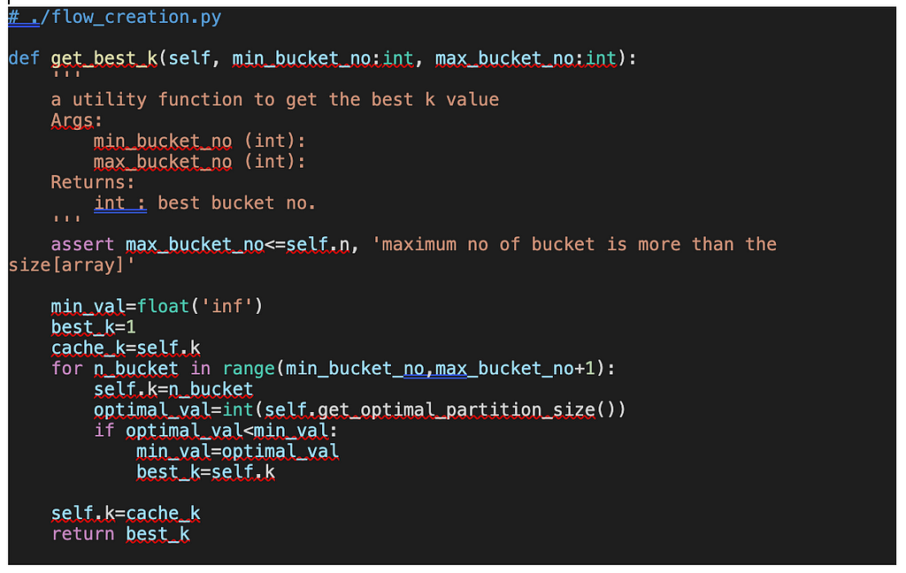
[Step — 3] We also have a useful function to get the best k value just for exploration. k value affects the parallelization of the flow and is usually decided based on the computing resource constraints.
Flow Chart:
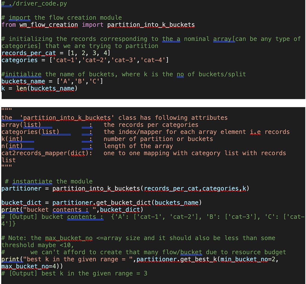
Below is the driver code to partition an array of records into k buckets:
Conclusion:
The blog started with the considerations to keep in mind while designing a ML workflow and presented a case where an algorithm was scaled to hundreds of categories across 5 countries using code and workflow node parallelization. Finally, we presented a code package to uniformly distribute input data across the different flows of a workflow. It presents an approach to developing a ML system that scales with minimal effort and is also easy to maintain. An approach like the one presented can help increase parallelization, reduce manual interventions and improve speed to market of an ML algorithm.
Automated Input Data Distribution In a Multinode Workflow was originally published in Walmart Global Tech Blog on Medium, where people are continuing the conversation by highlighting and responding to this story.