 https://www.pexels.com/ru-ru/photo/828658/
Introduction
As the largest grocer in the United States, Walmart has a massive assembly of supermarket refrigeration systems in its stores across the country. Food quality is an essential part of our customer experience and Walmart spends a considerable amount annually on maintenance of its vast portfolio of refrigeration systems. In an effort to improve the overall maintenance practices, we use preventative and proactive maintenance strategies. We at Walmart Global Tech use IoT data and build algorithms to study and proactively detect anomalous events in refrigeration systems at Walmart.
One of the key components in identifying refrigeration anomalies is defrost. A refrigeration system undergoes defrost periodically to get rid of frost and ice that gets built up during its normal operation. Depending on the type and its contents, a refrigeration case might undergo defrost multiple times in a day. During defrost, the refrigeration unit warms up and its temperature increases significantly above steady state. As a result, it becomes important to correctly identify if a rise in case temperature is due to an anomalous event or defrost.
In this blog, I will talk about a technique for identifying and predicting defrost in refrigeration cases using a concept known as Fourier Transform. The goal here is to introduce this concept at a high level, study a toy example with its python implementation and look at the methodology and results of our defrost prediction work.
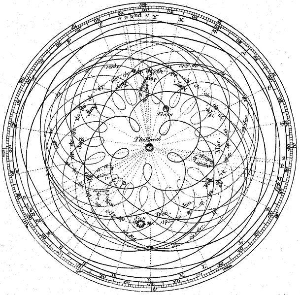
To understand the idea behind Fourier Transform, let us go back in history and visit one of the earliest mathematical models of the universe called — Ptolemaic system. Ptolemy, along with other Greek physicists, tried to model the universe with Earth at its center and planets moving around in circular motion. However, the paths of the Sun, Moon, planets and stars as observed from Earth are not circular. So Ptolemy added “eccentricity” to his models using the idea that — the planets move around in one big circle, but then also move around a little circle at the same time like a point on the edge of a wheel. This model still didn’t explain the planetary motion correctly and eventually it was refined by adding more circles on top of circles to look something like this:
 https://math.stackexchange.com/questions/1002/fourier-transform-for-dummies
In present times we know that this concept is not accurate and planetary motion is more complex than combination of simple circles. However this Greek system demonstrates one powerful concept- we can approximate any curve by adding up enough circles of varying sizes and speeds. This idea forms the backbone of Fourier Transform : Any given signal can be split into a set of distinct circular paths.
Fun side-note : Drawing Homer Simpson’s face using Ptolemy’s system of epicycles : Ptolemy and Homer (Simpson)
Behind the curtains:
Now that we have a high level understanding of Fourier Transform, let’s dive deeper into how it works. Let’s start by looking at the features of a circular path. Any circular path can be described using three things — size, speed and starting angle. By varying these, we can create different circular motions.
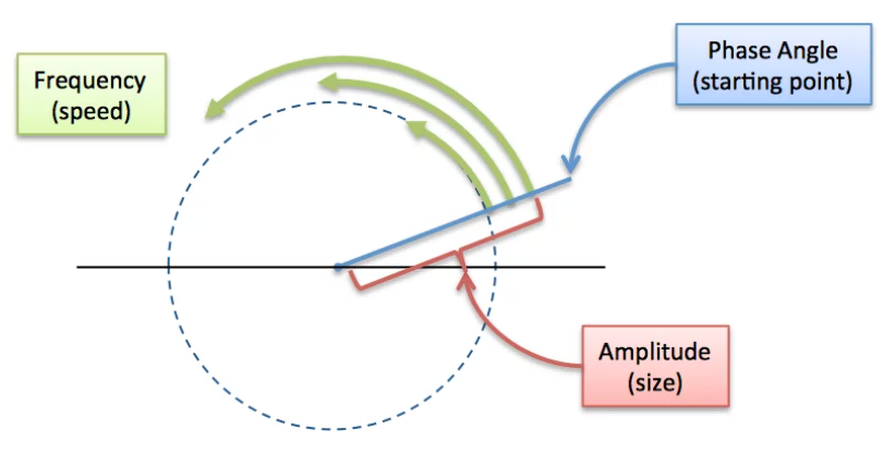
 Left: Describing a circular path. https://betterexplained.com/articles/an-interactive-guide-to-the-fourier-transform/. Right: If a time component (x_axis) is added to such a circular path, then we get a sinusoidal signal as shown. https://www.kdnuggets.com/2020/02/fourier-transformation-data-scientist.html
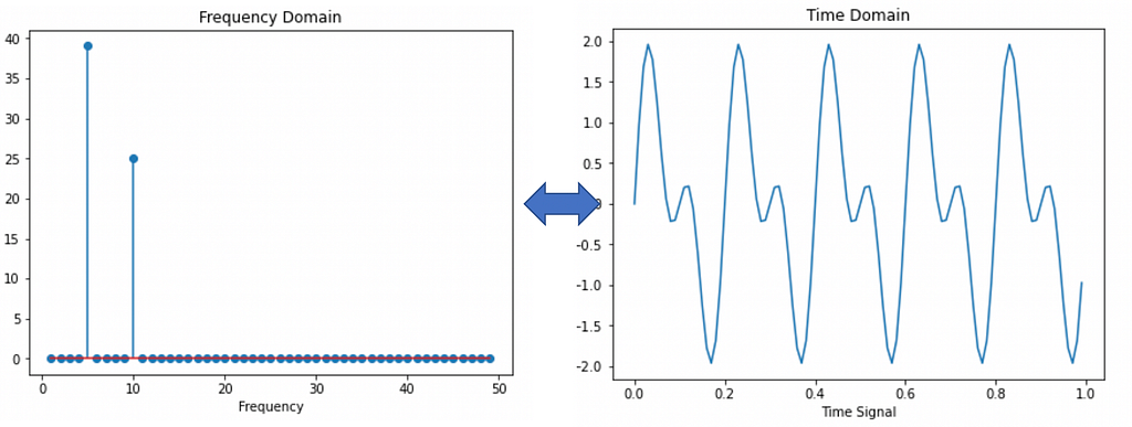
By mixing multiple such signals, we can create a complex signal. Looking at this the other way, we can say — Any signal can be approximated as a sum of sinusoidal signals with different frequencies. The Fourier Transform process does just this — it takes any signal and decomposes it into its constituent frequencies. In doing so, it converts a time-domain signal into frequency-domain.
To sum up, Fourier Transform decomposes a given time-based signal into a bunch of sinusoids with different speed, amplitude and phases. Mathematically, it can be represented like this.
 credit:https://www.thefouriertransform.com/series/fourier.php
The coefficients ak and bk will decide the relative importance of each of the sinusoidals in the series.The exact math can get hairy and we will avoid it for this blog.
From an implementation perspective, let us look at how to do this Python. We will create a simple sinusoidal signal and look at its frequency profile using FFT (FFT is faster implementation of Fourier Transform)
import numpy as np
import matplotlib.pyplot as plt
## Create a simple signal
# sampling rate and frequency
dt = 0.01
f = 10
t = np.arange(0,1,dt)
# signal
f = np.sin(2np.pift)
## Compute the Fast Fourier Transform (FFT)
n = len(t)
# Compute the FFT
fhat = np.fft.fft(f,n)
# Compute the Amplitude
A = fhat * np.conj(fhat) / n
# Create frequencies
freq = (1/(dtn)) * np.arange(n)
# Only plot the first half of freqs
l = np.arange(1,np.floor(n/2),dtype=‘int’)
## Plots
fig,axs = plt.subplots(1,2)
plt.sca(axs[0])
plt.plot(t,f)
plt.sca(axs[1])
plt.stem(freq[l],A[l])
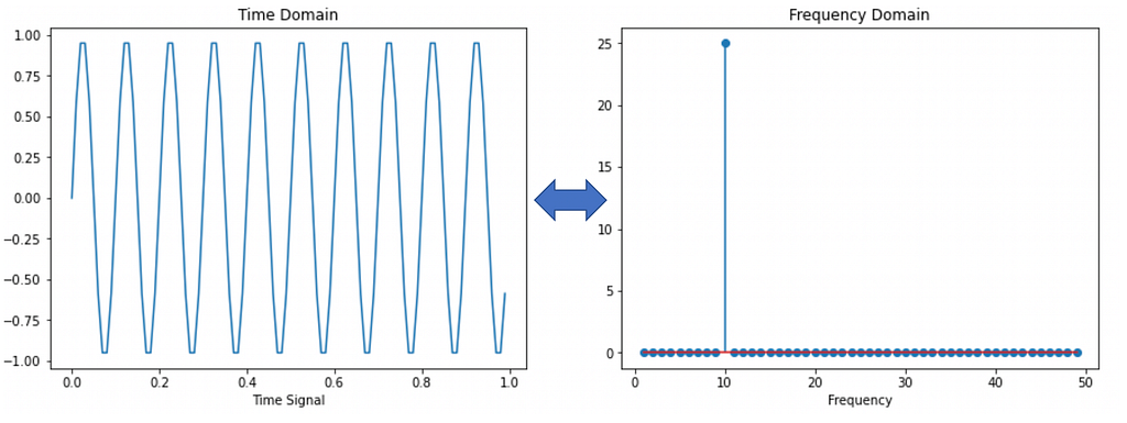 Left: Time domain signal. Right: Positive half of the Fourier Transformed signal. It can be verified that the signal is comprised of only 1 frequency and all others frequencies are zero. The frequency spectrum is symmetric around zero and contains both negative and positive frequencies as the output of Fourier Transform contains complex numbers. You can read more about it here : https://realpython.com/python-scipy-fft/
Similarly, by taking the inverse fourier transform, we can get a signal from frequency spectrum back the time domain signal
# Inverse FFT for filtered time signal
inv_fft = np.fft.ifft(fhat)
 Inverse Fourier Transform converts a signal in frequency domain back to time domain
In essence, using Fourier Transform, we can design a generic framework for signal processing like this:
- Take a time-based signal
- Split it into constituent sinusoidal signals
- Separate and analyze individual constituent signals as needed
Toy example : Denoising information signals
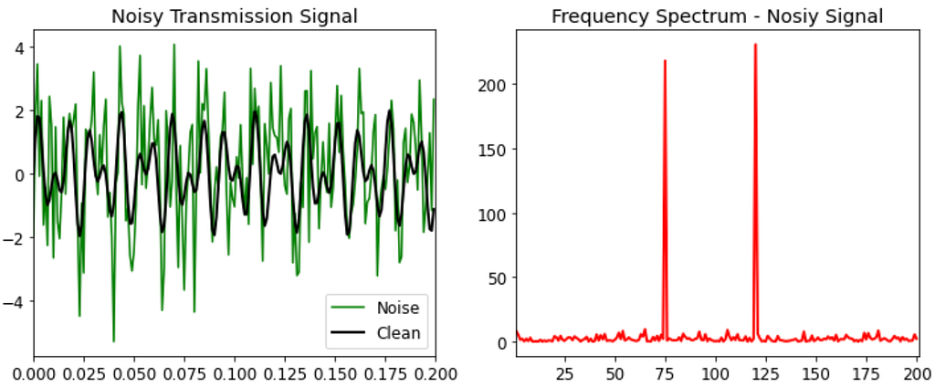
Let us extend our understanding of Fourier Transform as explained above and demonstrate how it can be used to solve a classical problem in information systems — signal denoising. In signal denoising, the goal is to retrieve the original information signal from a given transmission signal which will be corrupted with some noise in transit. We will try to achieve this using Fourier Transform. A key assumption that we make here is that the noisy transmission signal comprises of two things:
- High magnitude frequencies corresponding to the original clean signal
- Low magnitude and irregular frequencies corresponding to noise added to the signal
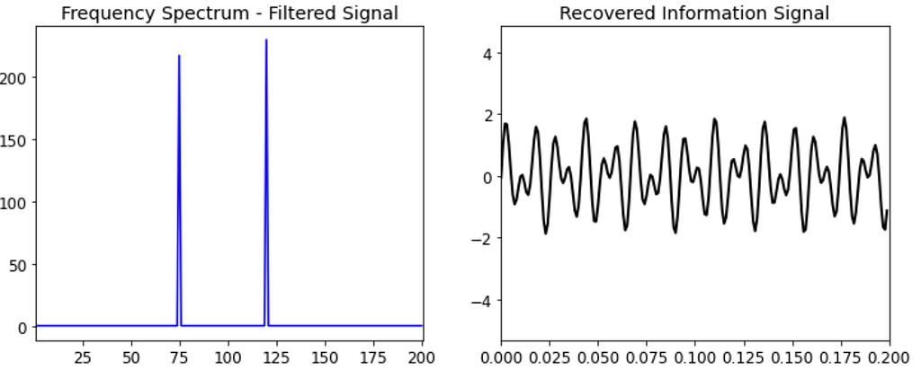
Once we make this assumption, then all that remains is filtering these low magnitude frequencies from the noisy signal to retrieve the original information content. This can be done in the following manner:
- Decompose the noisy signal from time domain into its constituent frequencies using Fourier transform
- Filter out all the low frequency components using a suitable threshold*
- Convert the filtered signal in frequency domain back to time domain using the inverse Fourier transform
threshold can be decided empirically or using domain knowledge.
import numpy as np
## Create a sample information signal as a sum of two frequencies
dt = 0.001
t = np.arange(0,1,dt)
f = np.sin(2np.pi75t) + np.sin(2np.pi120t)
f_clean = f
# Add some noise
f = f + 1.5np.random.randn(len(t))
## Compute the Fast Fourier Transform (FFT)
n = len(t)
# Compute the FFT
fhat = np.fft.fft(f,n)
# Compute the Amplitude
A = fhat * np.conj(fhat) / n
# Compute the frequencies
freq = (1/(dtn)) * np.arange(n)
# Create an index to filter large frequencies
idx = A >= 50
# Zero out smaller frequencies
fhat = idx * fhat
# Take inverse FFT to retrieve the original signal
inv_fft = np.fft.ifft(fhat)
Predicting Defrost in Refrigeration Cases at Walmart
Let’s circle back to our goal of predicting defrost periods in refrigeration cases. As described earlier, to be able to profile defrost in refrigeration cases is a key input in forecasting refrigeration anomalies. For the purpose of this blog, we will rely on univariate case temperature data of a refrigeration case.
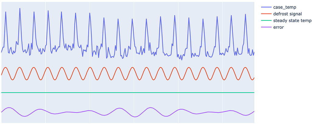 Typical temperature profile of a refrigeration case and how it can be thought of as a combination of defrost signal, steady state signal and random fluctuations (error).
The case temperature signal shown above is typical of refrigeration cases that need to maintain a steady temperature and undergo defrost periodically. The challenge here is that these defrost periods shift gradually over course of time depending on factors such as external weather, case contents, store traffic, repairs, etc. As a result, we need a robust logic to detect defrosts that are periodic in short term but slowly shifting on a longer time frame.
We will make use of Fourier Transform to process the case temperature signal and extract defrost signal from it. To do so, we simplify the case temperature as being composed of three parts : defrost, steady state temperature and error. Once we make this assumption, all that remains is filtering the frequency component that corresponds to defrost from the Fourier transformed temperature signal.
Below is a general outline of this process:
- Convert case temperature signal from time domain into frequency domain.
- Study the frequency spectrum and identify relevant components. For our use-case, we were able to identify that: steady state temperature had zero frequency (dc signal) and highest magnitude, and defrost signal belonged to frequency with second highest magnitude.
- Filter the frequency spectrum to contain only the frequency belonging to defrost and filter out the rest.
- Take Inverse Fourier Transform of the filtered frequency spectrum to get the defrost signal.
- Predict defrost periods in upcoming days by extrapolating the identified defrost signal.
# Function to extract defrost signal from case temperature data
def get_defrost(x):

    ## Calculate fast fourier transform
    fhat = np.fft.fft(x,len(x))
    A = fhat * np.conj(fhat) / len(x)
    ## Get the second highest amplitude in frequency domain
    #  that will belong to the defrost signal
    idx = A >= sorted(A)[-2]

    # filter out remaining frequencies
    fhat = idxfhat


    ## Inverse FFT to extract the defrost signal
    ffilt = np.fft.ifft(fhat)

    return abs(ffilt)
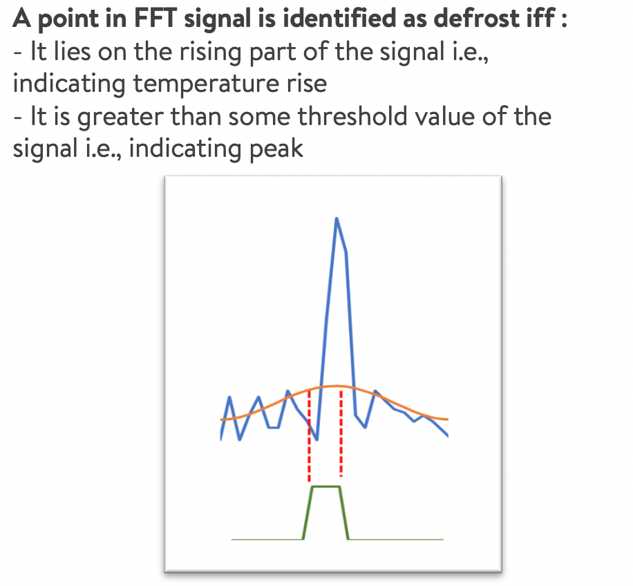
The extracted defrost signal needs to be converted into a binary indicator for downstream modelling. This can be done by thresholding the sinusoidal defrost signal at a suitable point and classifying the upper portion of the signal as defrost indicator. This threshold is a hyperparameter and in our case we decided to use the a suitable value after some experimentation.
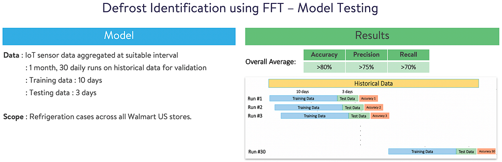
As noted earlier, we have a few refrigeration cases where the defrost command is accurate and readily available in IoT sensor data. We benchmarked our results against these cases. Below is the modelling setup and a few examples of good and bad model fit:
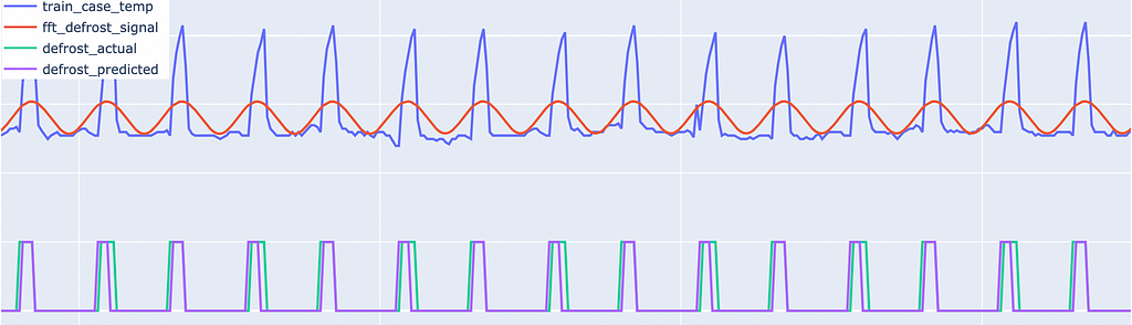 Example #1 : Good Model Fit
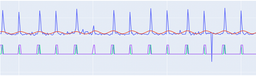 Example #2 : Bad Model Fit, Low Precision & Recall
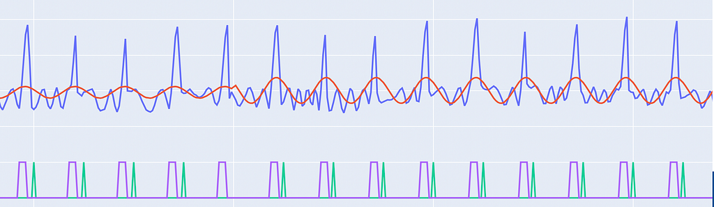 Example #3 : Bad Model Fit, Zero Precision & Zero Recall
Example #3 is particularly interesting as here it looks like the model performance is bad, but on inspection you can see it’s a data quality issue. Although the predicted defrost looks correct, the actual command is out of sync with the defrost cycle (it peaks after the defrost). Thus cases, where the model is performing really bad, can be considered as potential data quality issues and flagged for further inspection.
Overall, the initial results are encouraging and Fourier Transform seems to do a decent job in cases where defrost periods are regular. In such cases, precision and recall are >80% on an average. The performance is low for cases where defrosts are aperiodic or lack general pattern. Here we will build on top of the current logic using a customised approach based on refrigeration case type, contents and inputs from domain experts.
To conclude, the current approach allows us to do the following :
- Generate defrost command for cases where the command is not readily available in data
- Predict future defrost schedule
- Identify and correct historical defrost command for cases where defrost command in IoT data is inaccurate
References
An Interactive Guide To The Fourier Transform
Denoising Data with FFT [Python]- https://www.youtube.com/watch?v=s2K1JfNR7Sc
But what is the Fourier Transform? A visual introduction- https://www.youtube.com/watch?v=spUNpyF58BY
Predicting Defrost in Refrigeration Cases at Walmart using Fourier Transform was originally published in Walmart Global Tech Blog on Medium, where people are continuing the conversation by highlighting and responding to this story.