 Image Source: Pixabay
Data involving any type of the specific geographical area or location information is called “spatial” data (or “geospatial” data). Geospatial data helps in understanding relationships between geographic attributes and any other metrics data, e.g., how does sales of product vary from urban areas to coastal areas? Geospatial data has various applications, such as
- Visualizing the area that the data describes
- Performing trade area analysis
- Selecting locations for opening new stores for a brand
- Planning telecommunication/transportation network
- Risk assessment due to destructive weather, etc.
Obtaining such insights are valuable which makes spatial data skills a great addition to any data scientist’s toolset. In this article, an introductory overview to Python’s spatial analytics ecosystem is provided through some fundamental geospatial operations from ‘geopandas’ package. By the end of this article, readers will learn about
- Basics of geospatial data format
- Creating a point geometry from latitude and longitude
- Creating buffer area around a point for trade analysis
- Visualizing geospatial data using folium
- Join operation between two spatial dataframes for intersecting points
1. Working with Geospatial Data
1.1. Vector Data
Vector data represent geometries in the world. When you open a navigation map, you see vector data. The road network, the buildings, the restaurants, and ATMs are all vectors with their associated attributes. Vector data is simply a collection of discrete locations ((x, y) values) called “vertices” that define one of three shapes:
- Point: a single (x, y) point. Like the location of your house.
- Line: two or more connected (x, y) points. Like a road.
- Polygon: three or more (x, y) points connected and closed. Like a lake, or the border of a country.
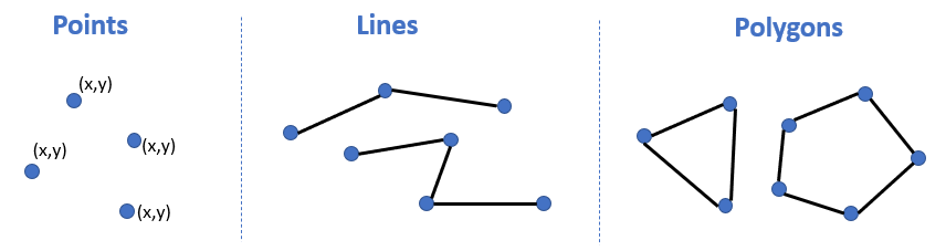 Shapes of different vector data
Vector data is commonly stored in a “shapefile” format. A shapefile is composed of three required files with the same prefix (here, ‘spatial-data’) but different extensions:
- spatial-data.shp: main file that stores records of each shape geometries
- spatial-data.shx: index of how the geometries in the main file relate to one-another
- spatial-data.dbf: attributes of each record
There are other file-types for storing vector data too like geojson. These files can generally be imported into Python using the same methods and packages we use below.
1.2. Geopandas
In this article, we will be primarily using open-source python library called geopandas to work with vector data in python. Geopandas extends the pandas capabilities to geospatial data and leverages the capabilities of shapely to perform geometric operations on spatial data. Geopandas depends on fiona for file access and matplotlib for plotting. Key datatypes used in geopandas are GeoSeries and GeoDataFrame like Series and DataFrames from Pandas. GeoDataFrames contain geometric column generally called as ‘geometry’. Geometry column contains different geometries like points (latitudes and longitudes), lines, polygons, etc., as shapely objects. Below is schematic view of a GeoDataFrame.
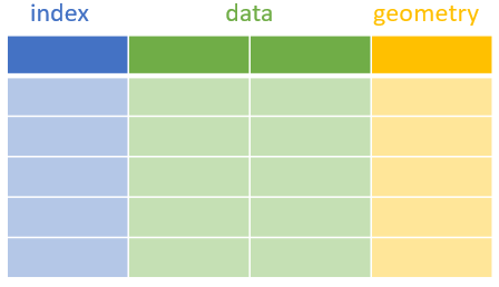 Data format of a typical geodataframe
Next, we will explore some examples of geospatial operations by analyzing a dataset on US fast food restaurants.
2. US Fast Food Case Study
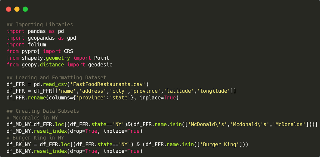
In this case study, we’ll be using a dataset from Kaggle which contains information about 10,000 fast-food restaurants in US. For the sake of simplicity, we will only analyze a subset of the dataset. The objective is to locate all the McDonald’s restaurants in New York state and determine how many Burger King restaurants (a competitor of McDonald’s) are in the vicinity of corresponding McDonald’s restaurants.
First, we’ll import the necessary python libraries and load the dataset.
2.1. Creating Point and Buffer Area
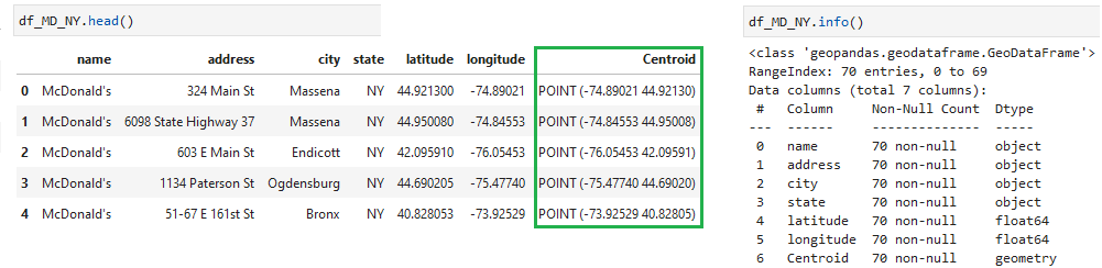
Note that these datasets are the usual Pandas dataframes. Next, we will convert these into geodataframes by creating a point geometry object from latitude and longitude. The following function uses the Coordinate Reference System (CRS) of WGS84 for converting the dataset into geospataial data. WGS84 is standard for GPS and is made up of a reference ellipsoid, a standard coordinate system, altitude data, and a geoid. The readers are encouraged to check this link to learn more about CRS.
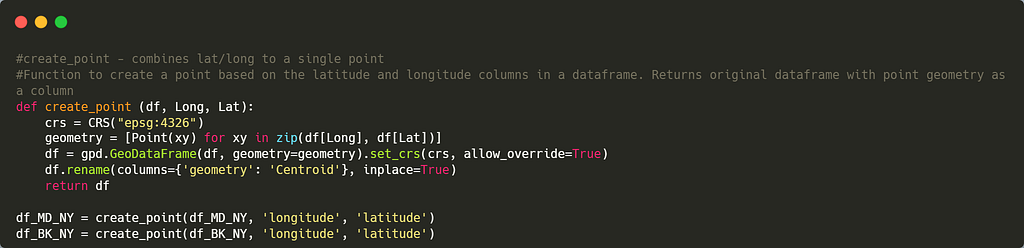
As it can be seen below, a new column ‘Centroid’ has been created which is a Point geometry data type and the class of the dataframe is converted to GeoDataFrame.
Next, we create a buffer area around the centroid points based on a given radius.
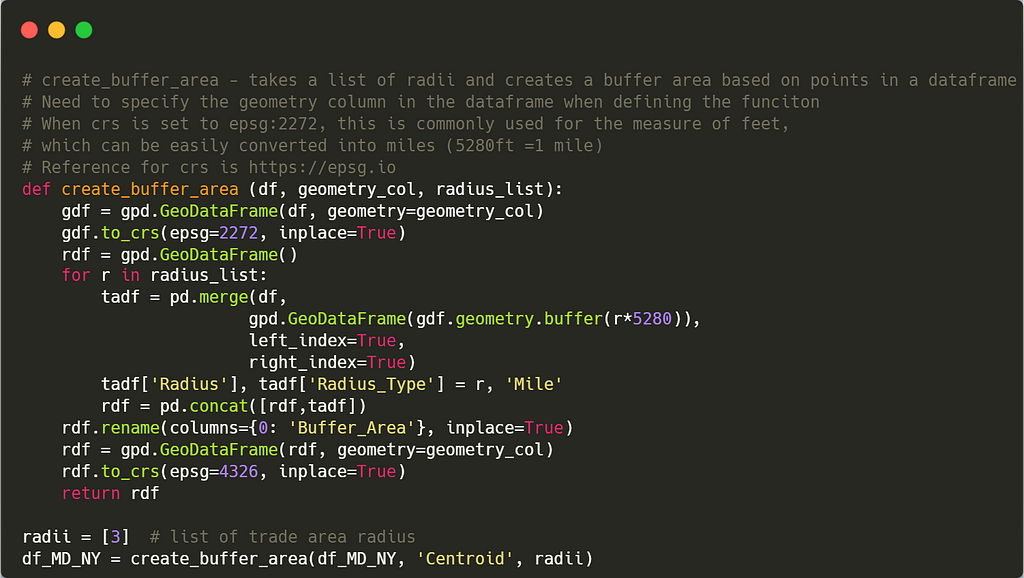
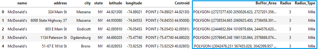
As shown below, the GeoDataFrame now consists of another geometry object column named ‘Buffer_Area’ which is a polygon.
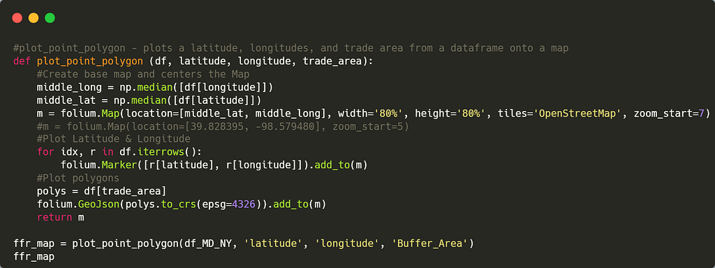
2.2. Visualizing Geospatial Data
Now, we are going to visualize both the point (‘Centroid’) and polygon (‘Buffer_Area’) geometry objects on a map using the python library ‘Folium’ and the underlying built-in tile-set ‘OpenStreetMap’.
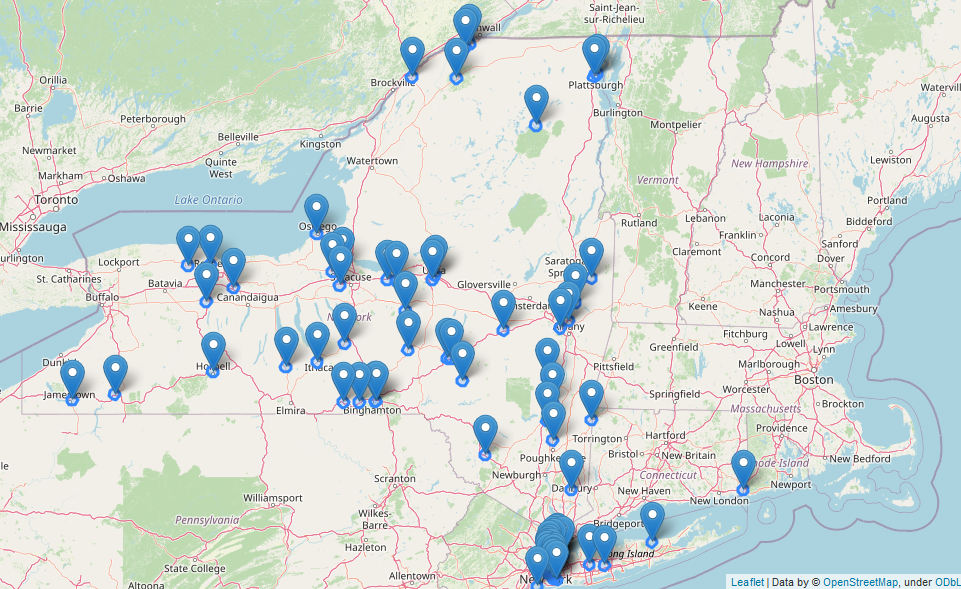 McDonald’s in New York State
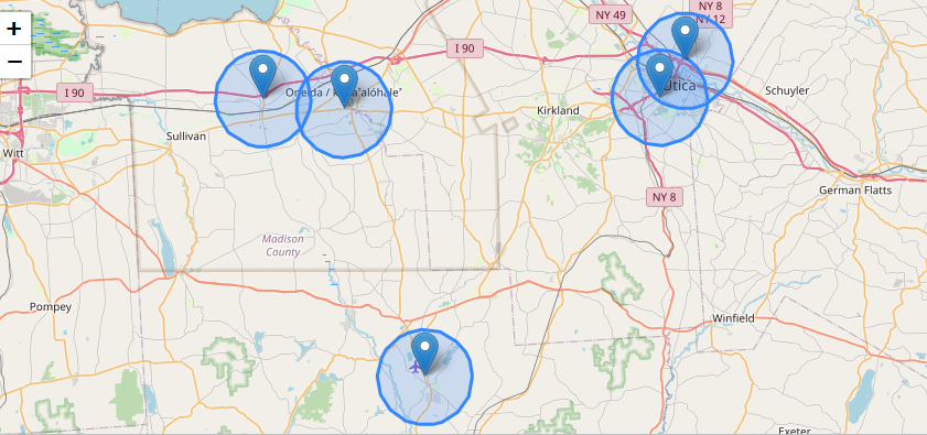 Polygons are drawn around 3 miles from all the McDonald’s
2.3. Spatial Join
In this section, we will find the Burger King restaurant points that fall within corresponding buffer areas of the McDonalds’ using Geopandas’ spatial join function. Just like Pandas’ join operation, this one also involves joining two geodataframes both having at least one geometry type variable. However, there are a few additional things that are noteworthy to mention:
- CRS units for geometry objects from both dataframes should match.
- The geometry objects in each data frame to be joined should both be named ‘geometry’ or ‘set_geometry’ options should be used to denote the primary geometry object in case there are multiple geometry columns in the dataframe.
- After performing the inner spatial join operation, only the geometry object data from the left data frame is retained and the other one is discarded.
For details, readers are requested to check the geopandas documentation here. The code below demonstrates how to use spatial_match to find the Burger Kings that are located within 3 miles of McDonald’s in New York.
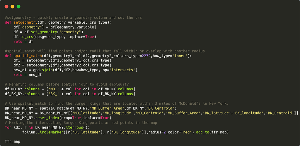
As it can be seen below in the zoomed-in version of the map, the Burger Kings are marked as red points within the blue buffer area of McDonalds’.
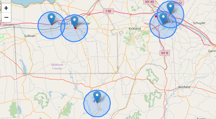 Red points indicate the locations of Burger Kings
The code for this case study can be found in this github link.
3. Conclusion
Goal of this article was to introduce the concept of geospatial analysis, geopandas and other resourceful open-source python spatial libraries. We have covered common spatial operations like creating geometry points, creating buffer areas, spatial joins, and visualizing geospatial data on maps. There is a lot more that can be done with geospatial analysis like creating the KML files from geospatial data, calculating drive distance between geo points, etc., which we would like to cover in future posts. So stay tuned.
Acknowledgment: Thanks to @Sai Manikanta Mukka for collaborating on this article.
4. References
- GeoPandas 0.11.0 - GeoPandas 0.11.0+0.g1977b50.dirty documentation
- The Shapely User Manual - Shapely 1.8.4 documentation
- 1 The Fiona User Manual - Fiona 2.0dev documentation
- Folium - Folium 0.12.1 documentation
- Fast Food Restaurants Across America
- OpenStreetMap
- EPSG.io: Coordinate Systems Worldwide
Introduction to Spatial Analytics in Python was originally published in Walmart Global Tech Blog on Medium, where people are continuing the conversation by highlighting and responding to this story.
Article Link: Introduction to Spatial Analytics in Python | by Samrat Nath | Walmart Global Tech Blog | Sep, 2022 | Medium