
Introduction
Linear optimization is a branch of optimization techniques where the goal is to find the best possible outcome based on a linear relationship between some constraints and an objective function. A wide variety of real-world use cases can be easily solved by formulating as a linear optimization problem. Typically, optimization includes finding the maximum or minimum value of an objective function that calculates cost, time, resources, etc. This objective function is evaluated in presence of certain constraints which must not be violated. In most of the cases, these constraints are hard constraints i.e their values are fixed and/or bounded.
Let us understand this more in detail with a small example. In figure 1, we present a use case where a company wants to assign vendors to carry out certain projects at the lowest possible cost. There are a fixed number of projects, and a fixed capacity and cost per project associated with each vendor. Using simple linear optimization, all the projects can be allocated at a total cost of $795. This is an example of using hard constrains — the capacity and cost numbers are fixed, and optimal solution is found within these bounds.
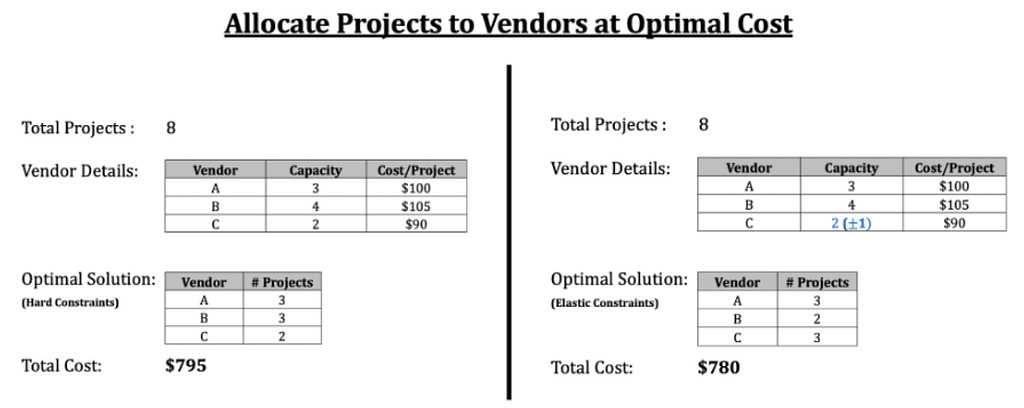
However, if we are allowed to play around with these constraints, we might get a different solution. As you can see on the right, if we increase the capacity of Vendor C by 1, we can now do the allocation at a reduced total cost of $780. Here, we have made one of the constraints elastic i.e. they are not fixed anymore and can violate their initial bounds by some margin. This is also reflective of what happens in an actual scenario during planning, the company might realize that Vendor C is more cost effective and will try to negotiate more capacity from them.
Thus, although an out-of-the-box optimization framework might work well for a lot of use-cases, there is always a risk that the optimizer will be restricted by the fixed number of the inputs. This happens because the algorithm is trying to find the optimal solution within the given set of constraints (fixed pre-conditions) such as — project schedule, vendor availability, vendor capacity, costs, etc. However, in real-world situations, these constraints are flexible and can be altered to suit the objective. For e.g., we can always ask a cost-effective vendor to increase their capacity or negotiate price with a long-term vendor to reduce costs.
Linear Optimization has worked great for a variety of our use-cases at Walmart. One such use-case is assigning 3rd party vendors for construction projects activities across our stores. Here, different vendors submit their bids for the projects and the aim is to assign a vendor to each project so that the overall cost is minimized while also considering factors like vendor ranking, vendor capacity etc. To solve for this, often a linear optimization model is sufficient, but the assignment may not always be perfect. Some of the reasons for this are:
- Cost of project is more than planned budget,
- Number of projects is greater than capacity of vendors,
- Scheduling of projects conflicts with vendor availability, etc.
In order to find an optimal and a realistic solution, we need to add some flexibility or elasticity to our model constraints. With a little experimentation, the end-user will be able to better understand the optimization results and effectively plan their assignment. Thus, a simple linear optimization framework can be thought of as a scenario planning tool for improved results by having flexible or elastic constraints.
In this blog, we will introduce the concept of Elastic Constraints in Linear Optimization and implement a toy solution in Python.
Math behind it!
In linear programming, whenever we are trying to solve constraints, we tend to have hard-bounded constraints. In many situations these constraints can be relaxed slightly depending on the context. We will now look at the math behind how to introduce soft (elastic) constraints into our framework.
Let us assume we have ’n’ stores where n>0 is a natural number. Each store needs to hire a manager from a third-party company. There are various companies providing this service with each company having a capacity (based on previous reputation and actual man resource availability) on how many resources they can provide. Each store needs one manager at most. Every third-party company submits their bid. The goal is to optimally allocate resources to all stores while minimizing the cost considering the capacity of each company.
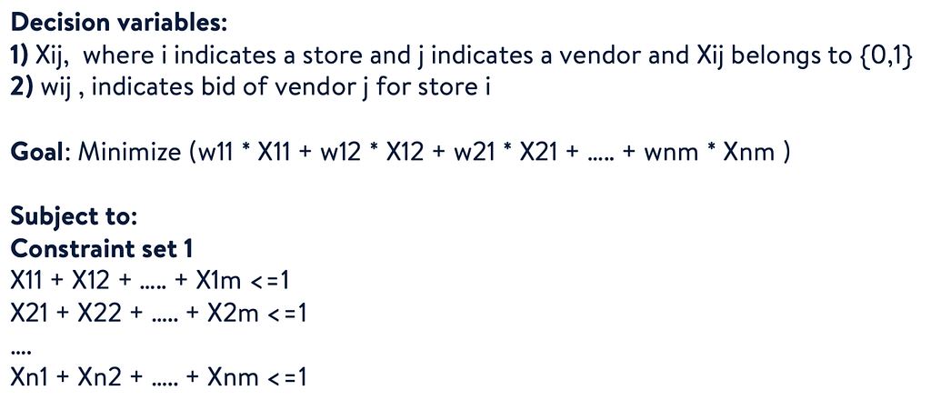
Every store should be allocated at most 1 vendor. Here we could have taken an equality constraint. However, if vendor capacity is less than the resources needed, putting equality constraint yields an infeasible solution. To overcome this challenge, we introduce <= constraints.
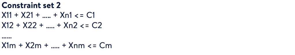
The total assignment to a vendor should be less than or equal to their capacity.
Elastic Constraints:
In many situations, it might be interesting to look at how the optimal solution will change if we loosen the constraints slightly. For e.g: If we loosen the vendor capacity by 10 %, by how much can we reduce our total cost? Or if we are unable to get full assignment with existing constraints, how does the assignment change if we loosen the constraints both in terms of resources and cost per project? In many situations this will help business make better decisions regarding the optimal allocation.
Let us now understand how to add elastic constraints to our optimization framework. We will be using the PuLP library in Python and it has 2 key arguments: Free Bound and Penalty.
Free bound:
Free bound represents a region around where we can allow the constraint to deviate freely from its initial fixed bound.
For example,
If we have x + y = 200, as a constraint
With a free bound of 1%, we can permit the value of x + y to be in the interval [198,202].
These bounds do not have to be symmetric. One can opt for different percentages on either side. This becomes important because we might not want to deviate from the constraint from one side. Let us say we never want to exceed 200, in that case we can set the right hand bound to 0%.
Any constraint value within this free bound is permissible. The concept can easily be extended to inequality constraints. Note, for inequality constraints one side is always a free bound. Namely, for ‘<=’, left is always a free bound and we can choose the right hand bound. A free bound of 0 indicates we do not allow the constraint to deviate from the value freely.
Penalty function:
The penalty function represents a way of introducing soft constraints in Linear Programming. Conceptually whenever we deviate from the constraint value/ free bound region, the solution is penalized by changing the objective function.
Let ‘p’ represent the unit penalty
Original Problem:
Maximize : (2x + 3y)
Subject to : X + y = 20
Transformed problem:
Maximize : (-p* rn + p* rp + 2x + 3y)
Subject to : x + y + rp + rn = 20
Where rp and rn represent continuous variables indicating positive & negative deviation from the constraint value. For every unit deviation r, we penalize the objective function by p making the total penalty rp.
Choosing p becomes a problem specific to the domain and problem statement. If the value of p is large, there is a very high per unit penalty hence making it hard to deviate from the original constraint value. Similarly, a low value of p indicates we can freely deviate from the constraint value.
As a rule of thumb, when we have a maximization problem, the penalty must be negative. In a minimization problem, the penalty must be positive.
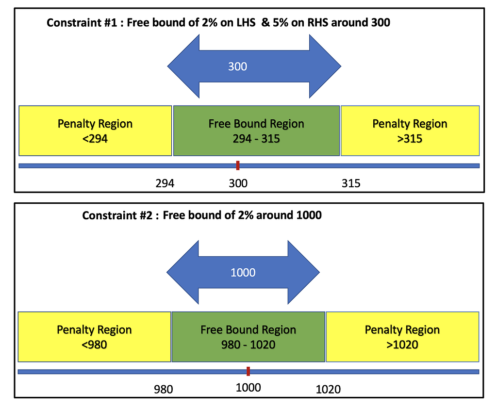
Sample Elastic Constraints in PuLP:
con_1 = LpConstraint(‘con_1’,sense=0,rhs=300)
elastic_con_1 = con_1.makeElasticSubproblem(penalty=1, proportionFreeBound = [0.02,0.05])
con_2 = LpConstraint(‘con_2’,sense=1,rhs=1000)
elastic_con_2 = con_2.makeElasticSubproblem(penalty=1,proportionFreeBoundList = 0.02)
Python Implementation
We will now look at the python implementation of the toy problem we discussed above:
# Import relevant functions from Pulp
from pulp import LpMaximize, LpProblem, LpStatus, lpSum, LpVariable, LpConstraint
Note: The original problem was a cost minimization problem where we wanted to assign one resource to every store. However, when we have fewer resources than stores, we will get an infeasible solution. To counter that we can change the equality constraints for stores to inequality (<=) constraints. But this leads to a solution where minimal is achieved by making every selection variable as 0. To ensure we can assign vendors to as many stores as possible, we convert this minimization problem into a maximization problem by changing the cost function. We subtract the bid amount from a large number and then maximize the problem as shown below:
# Vendor Details
# We are considering 3 vendors to be assigned to 8 stores
vendors = [‘A’, ‘B’, ‘C’]capacity = {‘A’: 2,
         ‘B’: 3,
         ‘C’: 1}bids = {‘A’: 100,
         ‘B’: 105,
         ‘C’: 90}
# Subtract bid amount from a large number, in this case: 1000
new_bids = {‘A’: 900,
         ‘B’: 895,
         ‘C’: 910}
Define the variables and the constraints
## Assignment Variables
# 3 vendors x 8 stores = 24 variables
x1 = LpVariable(‘1A’,lowBound=0, upBound=1, cat=‘Integer’)
x2 = LpVariable(‘2B’,lowBound=0, upBound=1, cat=‘Integer’)
x3 = LpVariable(‘3C’,lowBound=0, upBound=1, cat=‘Integer’)
x4 = LpVariable(‘4A’,lowBound=0, upBound=1, cat=‘Integer’)
x5 = LpVariable(‘5B’,lowBound=0, upBound=1, cat=‘Integer’)
x6 = LpVariable(‘6C’,lowBound=0, upBound=1, cat=‘Integer’)
x7 = LpVariable(‘7A’,lowBound=0, upBound=1, cat=‘Integer’)
x8 = LpVariable(‘8B’,lowBound=0, upBound=1, cat=‘Integer’)
x9 = LpVariable(‘9C’,lowBound=0, upBound=1, cat=‘Integer’)
x10 = LpVariable(‘10A’,lowBound=0, upBound=1, cat=‘Integer’)
x11 = LpVariable(‘11B’,lowBound=0, upBound=1, cat=‘Integer’)
x12 = LpVariable(‘12C’,lowBound=0, upBound=1, cat=‘Integer’)
x13 = LpVariable(‘13A’,lowBound=0, upBound=1, cat=‘Integer’)
x14 = LpVariable(‘14B’,lowBound=0, upBound=1, cat=‘Integer’)
x15 = LpVariable(‘15C’,lowBound=0, upBound=1, cat=‘Integer’)
x16 = LpVariable(‘16A’,lowBound=0, upBound=1, cat=‘Integer’)
x17 = LpVariable(‘17B’,lowBound=0, upBound=1, cat=‘Integer’)
x18 = LpVariable(‘18C’,lowBound=0, upBound=1, cat=‘Integer’)
x19 = LpVariable(‘19A’,lowBound=0, upBound=1, cat=‘Integer’)
x20 = LpVariable(‘20B’,lowBound=0, upBound=1, cat=‘Integer’)
x21 = LpVariable(‘21C’,lowBound=0, upBound=1, cat=‘Integer’)
x22 = LpVariable(‘22A’,lowBound=0, upBound=1, cat=‘Integer’)
x23 = LpVariable(‘23B’,lowBound=0, upBound=1, cat=‘Integer’)
x24 = LpVariable(‘24C’,lowBound=0, upBound=1, cat=‘Integer’)
## Constraints# Store assignment
# Each Store must have at most 1 vendor assigned
model += (x1+x2+x3<=1)
model += (x4+x5+x6<=1)
model += (x7+x8+x9<=1)
model += (x10+x11+x12<=1)
model += (x13+x14+x15<=1)
model += (x16+x17+x18<=1)
model += (x19+x20+x21<=1)
model += (x22+x23+x24<=1)
# Objective Function
model += (900x1+900x4+900x7+900x10+900x13+900x16+900x19+900x22+<br />         895x2+895x5+895x8+895x11+895x14+895x17+895x20+895x23+<br />         910x3+910x6+910x9+910x12+910x15+910x18+910x21+910*x24)
In PuLP, the way to introduce elasticity is to first define the object function and then extend it to include the elastic constraints. This is actually knows as adding soft constraints to the model. Optimization with elastic constraints is equivalent to adding a subproblem to the main objective function with some additional penalty.
Note: As explained previously, the choice of free bound region and penalty is use-case specific. For simulating elasticity, select these values such that the optimizer is forced to operate only within the free bound and incurs a heavy penalty if it goes beyond. For our use-case, we select a penalty of -100 for all vendors. As it is a maximization problem, the optimizer stays within the free bound to avoid the reduction in objective function.
# Adding Elastic Constraints
# For vendor A, we define an elastic constraints with a free bound range of +50% and penalty of -100
els_v1 = lpSum([x1,x4,x7,x10,x13,x16,x19,x22])
els_v1_con = LpConstraint(e=els_v1, sense=-1, name=‘elastic_v1_con’, rhs=2)
els_con1 = els_v1_con.makeElasticSubProblem(penalty=-100, proportionFreeBound = 0.5)
# For vendor B, we define an elastic constraints with a free bound range of +50% and penalty of -100
els_v2 = lpSum([x2,x5,x8,x11,x14,x17,x20,x23])
els_v2_con = LpConstraint(e=els_v2, sense=-1, name=‘elastic_v2_con’, rhs=3)
els_con2 = els_v2_con.makeElasticSubProblem(penalty=-100, proportionFreeBound = 0.5)
# For vendor C, we define an elastic constraints with a free bound range of +100% and penalty of -100
els_v3 = lpSum([x3,x6,x9,x12,x15,x18,x21,x24])
els_v3_con = LpConstraint(e=els_v3, sense=-1, name=‘elastic_v3_con’, rhs=1)
els_con3 = els_v3_con.makeElasticSubProblem(penalty=-100, proportionFreeBound = 1)
model.extend(els_con1)
model.extend(els_con2)
model.extend(els_con3)
model
Now, solve for optimal solution
# Solve the problem
status = model.solve()
Look at the assignment variables
print(f"status: {model.status}, {LpStatus[model.status]}")
print(f"objective: {model.objective.value()}")
for var in model.variables():
    print(f"{var.name}: {var.value()}")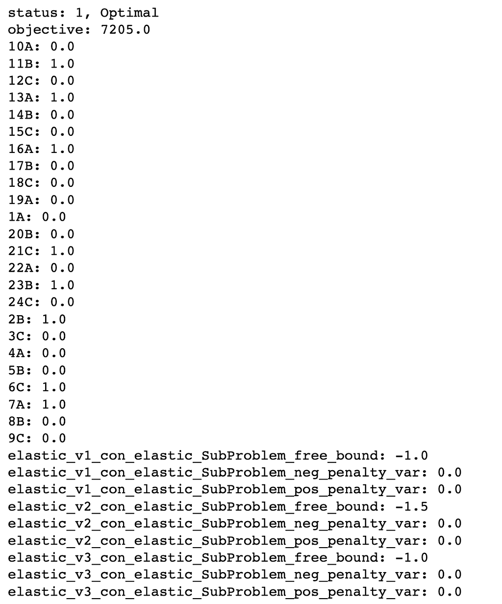
Scenario Planning
Let’s circle back to our goal of adding elasticity to our vendor assignment use-case. The two key results of assignment are : Total Cost, & Number of Assignments. Below is an example of how the optimization works out for a sample of 100 projects.
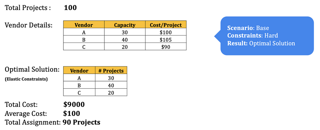 Simple Linear Optimization
We can see that in this base scenario, out of 100 projects, only 90 have been assigned because the total available vendor capacity is low. However, we need to ensure all of our projects are staffed. To achieve this, we can make the vendor capacities elastic and simulate scenarios to see how the assignment changes. Below are 3 examples where both — the cost and the assignment varies between different scenarios.
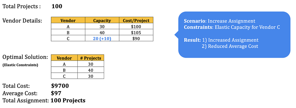 Scenario #1
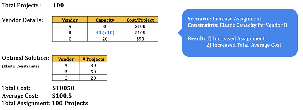 Scenario #2
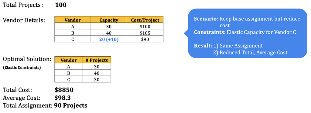 Scenario #3
As shown in the above examples, playing with vendor capacity can lead to various situations where we can see how the average cost & total assignment changes with a change in the capacity. This helps business make a much more informed decision compared to situation with fixed constraint and one allocation. We can also play with penalty function and free bound to create scenarios and cater to problems according to business needs.
Conclusion
We introduced the concept of elastic constraints and its implementation in Python. Further, we also looked at how it adds an element of scenario planning to our optimization framework and help plan more efficiently. This is a generic framework that can be introduced in any kind of linear programming problem and has a lot of applications specially in cases where the constraints are man-made and can be flexible. This is also a parametric approach which allows the inputs (essentially free bound and penalty) to be driven and selected by the person running the optimization making it ideal for scenario planning. We hope this blog has given you a fundamental idea on the concept and ideas on adding more power to your optimization use-cases.
Written by :
- Mandeep Singh (Mandeep Singh)— Data Scientist, Walmart Global Tech
- Sujay Madbhavi (Sujay Madbhavi) — Data Scientist, Walmart Global Tech
References
- pulp: Pulp classes - PuLP v1.4.6 documentation
- An example of soft constraints in linear programming
- Elastic Constraints - PuLP 2.6.0 documentation
Notes — https://www.cis.upenn.edu/~danroth/Talks/soft-constraints-ilp-VS-2013.pdf
Notes — https://www.csl.cornell.edu/~zhiruz/pdfs/softsched-iccad2009.pdf
Fine Tuning Optimization Results with Scenario Planning using Elastic Constraints was originally published in Walmart Global Tech Blog on Medium, where people are continuing the conversation by highlighting and responding to this story.