Forecasting is one of the most frequently requested machine-learning functions from Walmart businesses. While different teams work in silo building ML models, often they use the same set of open-source packages, repeating the efforts endlessly. Recently, we have developed a reusable forecasting library (RFL) to circumvent this situation with a design that eyes on scalability and extensibility at the same time.
Requirements
We started out with a requirement that RFL must be configuration-based. The application dependent information is specified in JSON files, while application agnostic part is implemented in the core library. This is motivated by our vision of Forecasting-As-A-Service where the front-end UI communicate with the back-end FAAS via JSON files which gives data owners from the businesses the opportunity to try what-if scenarios in a no-code fashion.
A second requirement is Extensibility. This includes the abilities of adding new forecasting models that are not currently in the library, and extending functionalities such as classification. RFL should make such kind of functional advancement straightforward to accomplish.
The final requirement is Scalability. In the projects we’ve engaged, there are those involving a few hundreds of models (small), tens-of-thousands of models (medium) or millions of models (large). All these use cases should be supported and ideally configured by flipping a flag in the JSON file.
Design
Our approach is to first form an abstraction of the computational process of forecasting. Then we capture the abstraction using Object-Oriented-Design (OOD) concepts. Our intuition is that once captured, adding new models/functions becomes a matter of sub-classing (from base classes).
One abstraction is the separation of data and computing. In Fig. 1a, fields of the data frame comprise of four types:
- Time index — this is the timestamp of the data point.
- Target — this is the target to be predicted.
- Partitions — columns here in fact define a data grid each joint of which is associated with a time series from the data frame. Fig. 1a shows some examples. Partition columns are also called dimensions.
- Features — considered as drivers of the target variable and used to assist the forecasting. Again, Fig. 1a shows some example features.
Fig. 1b is an illustration of the computation that’s happening at the joint. It consists of a pipeline of stages which run sequentially, in many trials (think of hyper-parameter tuning). All pipelines run the same program but with different data (doesn’t it sound like a Single-Program-Multiple-Data thing?).
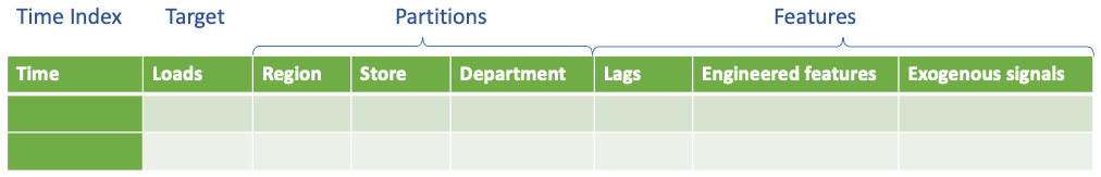 Figure 1a. Abstraction of data: think of data as multiple time series at the joints of the partition grid
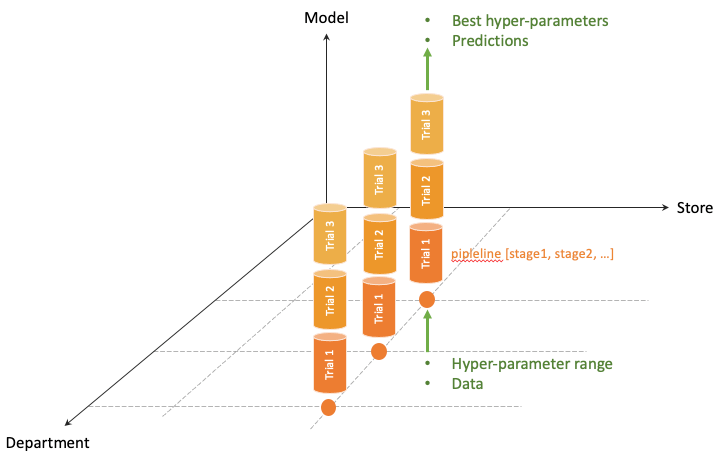 Figure 1b. Abstraction of computation: parallelization happens at joints and trials
The second abstraction looks further into the computing aspect (Fig. 1b). Here we observe the separation of the functionality that runs in the pipeline and the computational resources that are allocated for the execution. We call the latter Backend. More will be presented in a following section.
Before going into the detailed descriptions, let’s briefly introduce the UML terminologies that will be used to represent our design:
- Is-a: A Is-a B means A is a subclass of the base class B
- Has-a: A Has-a B means B is a member of A
- Uses-a: A Use-a B means A has a reference to an object of B, typically passed in as a parameter to a member function of A
Dataset reflects the data abstraction shown in Fig. 1a earlier. Out of the four types, we would like to concentrate our attention on features. Different types of features have different behaviors. It is best to capture them with an object-oriented design as depicted in Fig. 2. The base class is FeatureEngineering which has two member functions: impute() and extend(). The former fills any N/A values. The latter computes each feature’s future values. From FeatureEngineering, five specific features are sub-classed.
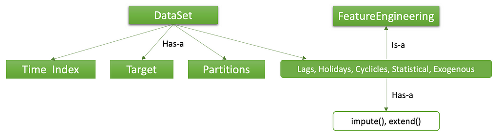 Figure 2. Hierarchy of the Dataset class
The Lags features are auto-regressive variations of the target itself, normally used in uni-variate models such as ARIMA. Holidays are easy to understand. Cyclicles encode temporal periods in weekly, monthly, quarterly and/or yearly frequency. They are similar to position encoding widely used in Transformer type NLP neural networks. Exogenous signals are external variables such as precipitation, unemployment, store foot traffic, etc. Statistical can be any arithmetic formula involving other features.
Function is where extensibility is achieved. In Fig. 3, the AutoPipeEstimator class is the provider of the functionalities. It accomplishes three things: i). incorporation of new forecasting models that are not currently in the library; ii). addition of new estimators such as classifiers; iii). adaptation to some popular machine learning API’s.
The SklearnEstimator class provides an example of API adaptation which in this case is Scikit-learn — a popular open-source ML package. The purpose of this adaptor is allowing RFL functions to be integrated into Scikit-learn pipelines as stages with other functions that follow the Scikit-learn coding convention. Pipeline is an efficient way of execution that is widely endorsed in the ML community. It eliminates transient data IO’s between the stages. Future extensions of new API’s can be implemented similarly.
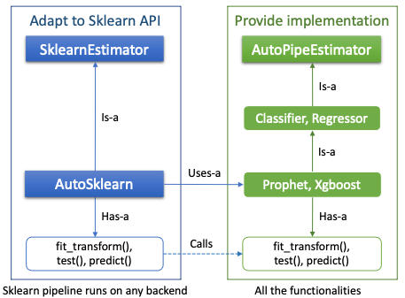 Figure 3. Hierarchy of the Function classes
Compute is a “pulling everything together” kind of class. It renders such a process: single Function is run against multiple data in Dataset on the scalable Back-end. So far, three back-ends are supported: Loop, Joblib and PySpark. The Loop back-end, by its name, is intended to run on a local computer in iterations of data. The Joblib back-end uses the Joblib open-source library for multi-threading. Finally, large-scale tasks can execute on a Spark cluster using the PySpark back-end.
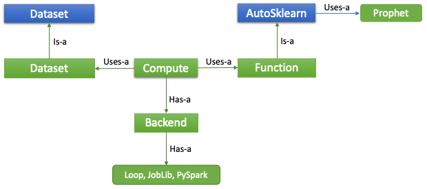 Figure 4. Hierarchy of the Compute class
Implementation
Runtime provides the top-level functions to the data scientists. For most of their daily duties, interaction with this class is granted sufficient. Four modes have been implemented: tune(), train(), test(), forecast() (Fig. 5). While it is possible for the data scientists to call these functions via the programming API’s, the standard way of usage is by configuration files where via the Config Handler class, the config info is loaded. Internally, the four modes call Compute to complete their assignment. The latter in turn passes the call to the actual Function object, a Prophet model, in this case. Incorporation of new modes in the future is painless thanks to the modular design. In terms of the configuration, Main config is for general settings and Model config for model specific settings.
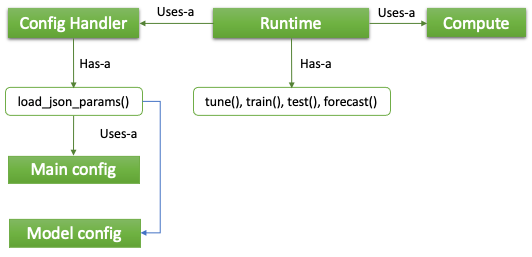 Figure 5. Runtime architecture
In addition to the four modes described above, RFL has some additional features that are worth mentioning here:
Recursive feature generation. It is necessary to generate future values of the exogenous signals and statistical features recursively in training and testing. For now, a vanilla Prophet model is utilized for this purpose. In case future values are available in the data frame, this functionality can be disabled in the configuration.
Grouping. There are use cases where the partition becomes overly granular, and the time-series signal becomes too sparse. A frequently encountered example is forecasting at the store-dept-category level. In such cases, data scientists would want to do a grouping first on some of the partition dimensions. RFL can be configured in a way that it trains a model on a group basis and generates forecasting for all partitions in the group.
Evaluation frequency. For performance evaluation of a model, different metrics are available such as MAPE, weighted MAPE, symmetric MAPE, MAE, etc. The evaluation can be made on an aggregated time series frequency instead of the dataset’s original one. This is especially important when the future time series has a different frequency, and the performance measures are to be compared when future data become available.
Summary
RFL has been adopted in several Walmart projects as the modeling tool. In summary, benefits reported from the data scientists are of two folds:
- Effort saving resulted from low code experiment setup. This amounts to 3–4 days saving and 90% execution time reduction due to in-build parallelization. With RFL, data scientists can focus more on designing the experiments rather than spending efforts in setting things up every time.
- Quality improvement afforded by wider exploration of hyper-parameter and feature spaces. While improving modeling quality is not a goal of the library itself, because of the simplification in experimentation, often data scientists do find more optimal models afterwards.
RFL is a reusable forecasting library designed with extensibility and scalability in mind. It is configuration driven as well— a design choice made to support our long-term vision of Forecasting-As-A-Service such that businesses as data owners can try what-if scenarios in a no-code fashion. In the future, we would like to promote its awareness within the company to increase further usages.
Acknowledgement
Multiple Walmart teams have participated in the development of NFL. Their contributions are acknowledged here all at once.
Design and Implementation of A Reusable Forecasting Library with Extensibility and Scalability was originally published in Walmart Global Tech Blog on Medium, where people are continuing the conversation by highlighting and responding to this story.