
Calibration is the process of transforming probability scores emitted out by a model so that their distribution match that which is observed in the training set(often unknown).
This article starts with a scenario in which calibration is desired and includes some real-world context around targeting in the Adtech(advertising technology) world. This section is followed by a mechanism to gauge the extent of calibration, then a way to calibrate the scores and a real-world application. The article ends with some endnotes.
Problem Statement
Machine learning(ML) models learn well if the training data is balanced, meaning, suppose if we want to train a model to classify an input image as either a cat’s or a dog’s image, then, ceteris paribus, the model will perform this task better if, during the training time, the data has nearly equal proportions of these two classes: cat and dog. So, if there is a huge class imbalance in the training data, then the classes are down-sampled before training the models. These models often arrive at intermediate real-valued scores(say, Probability[image is cat]=0.9) called prediction scores, and using these scores finally make the discrete predictions(cat/dog). The down-sampling changes the prior distributions in the training data and thus affects these posterior class probabilities. These scores do not indicate the true likelihood of an input point belonging to a predicted class and thus, there is scope for calibration!
If the requirement is just discrete predictions or ranking the input records using the intermediate scores, then calibration is not required even with the use of the down-sampling in the training. But, there are many scenarios where the intermediate scores which reflect the true likelihoods are desired. For example, to create bids for the auctions where advertisers compete to show advertisements to a customer, combining scores emitted by various models to arrive at a final prediction, communicating the true likelihood of the emitted predictions to estimate errors in prediction(how many of the images predicted by the models as cat’s images will indeed be cat’s images!), etc.
In the Adtech world, advertisers often need meaningful segments of the customers whom they can target via ads. These meaningful segments could be the sets of customers who are loyal to the brands of advertisers, who are not loyal (if the advertisers want to improve their incremental sales, they can target these folks), who are actively searching for a type of product (say, laptops), who will most probably buy an item in next few days, etc. The training data available to train models for creating the above segments often have huge class imbalances. The reason being among millions of customers you would find a very less proportion of customers who would have done the activity of the interest(mostly, purchase-activity) for a given advertiser. And thus we employ the down-sampling technique to train better models!
Many models trained with down-sampled-balanced data in a probabilistic framework such as Logistic Regression emit out these real-valued numbers which might not be calibrated. It means that if you look at the set of customers having prediction scores of 0.99, then you can’t say that 99% of those customers will belong to the positive class(or say, purchase from the brand). To arrive at such a statement, you first need to calibrate the scores to correct for the effect of the down-sampling. Then, you may find that the mean prediction scores of the above set of customers have reduced to 0.7 and now you can make a statement like 70% of these customers may convert!
In summary, calibration is required wherever you need the prediction scores to match the actual likelihood of the data points belonging to a given class. But first, how do we find if the scores are not calibrated? The next section provides the way!
How to figure out if the scores are not calibrated?
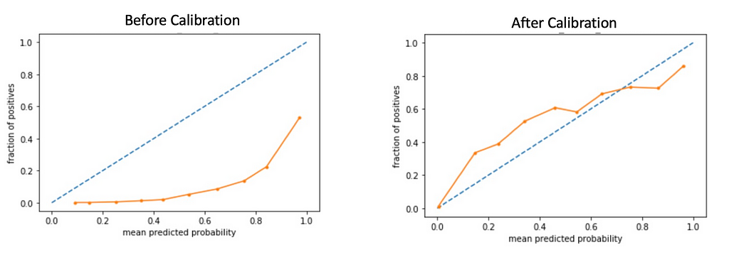
When the true probabilities are not known for real-world problems, the calibration can be visualized using reliability curves(Degroot & Fienberg, 1983). Before training the ML models, we often keep a small part of it as a holdout set(test set) and do not use it for training(train set), instead, we estimate the efficacy of the model trained using the train set by making predictions on the test set and comparing them with the known actual classes. In the test data(sampled before down-sampling), we have both actual classes and prediction scores from the model. Create a few bins of the prediction scores(say 10 bins between 0 and 1), and collect the set of customers falling in each bin based on their prediction scores. For each bin calculate x=mean-prediction-score and y = fraction-of-positives(class of interest, say “loyalist to a brand” ). Plot these points on a graph. For a well-calibrated scenario, the plot should be a straight line y=x.
 Calibration of the Prediction Scores
Here, calibration is the extent to which predicted probabilities are agreeing with the occurrence of positive cases. In the above figures, you can see that after calibration, the scores are aligning with y=x more than those before calibration. Of course, perfect calibration is wishful thinking given that there is a margin of error also in the trained model.
How to calibrate?
Pozzolo et al.(2015) proposed a way to calibrate the scores when the input training data to the model was down-sampled. Let’s understand this through an example:
In the training dataset(assume binary classification set up: there are two classes in the data only, say “loyal customers” and “non-loyal customers”):
- Total records: 300M
- The proportion of +ves in this original training set say ppos_o: 10% (and thus proportion of -ves, say pneg_o: 90%)
- We down-sample both +ves and –ves to take 1M each from both classes(tractable amount! otherwise it requires a lot of resources to train the model with 30M +ves and 30M -ves)
- So, in this balanced and down-sampled dataset, the proportion of +ves, say ppos_d is 50% (and thus the proportion of -ves, say pneg_d: 50%)
- We train an LR model on the balanced dataset, and for one record the model predicts 0.96 as the probability of being +ve, say probP_d. Thus, the uncalibrated probability of the input belonging to the negative class(say, probN_d) is 0.04. We get calibrated probability, say probP_o, as follows:
- probP_o = “(0.96)∗(0.1/0.5)” /( “(0.04)∗(0.9/0.5)”+ “(0.96)∗(0.1/0.5)” )= 0.73 (got scaled down from 0.96)
- We need to record the proportions of positive and negatives in the original training data and the down-sampled training data and the following formula helps us in calibrating the scores
 calibration formula
- The above expression(which has its roots in Bayes Minimum Risk Theory) shows that the output scores will be calibrated via upscaling/downscaling in the inverse proportions by which their respective classes were scaled in the down-sampling phase.
The above reference(Pozzolo et al.) suggests that if we choose positive-class-ratio-in-original-train-data(10% here) as the new threshold to assign the classes, it will give the same class predictions (discrete) as what we were getting with uncalibrated scores and threshold=0.5(positive class ratio in the balanced dataset). So, if we were choosing 0.5 as the threshold to classify a data point as belonging to the positive class, then with calibrated scores, the threshold should be adjusted to 0.1.
Real-World Application
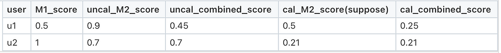
In this application, we demonstrate the need and advantage of calibration when the output of two models is combined to arrive at the final prediction score. Advertisers often ask for segments of customers loyal to their brands and who will purchase in the next few days. This ask is sometimes broken into two tractable ML problem statements: one ML model(say, M1) predicts the loyalty of a customer toward a brand, and another model(say, M2) predicts the probability of a customer purchasing an item from a given product type (say, “ shampoos” if this brand is selling shampoos) in next few days. To arrive at a final score for a customer, we combine(say, multiply) the scores from the two models and then rank the customers to create segments. Now, it’s important to calibrate the scores of the two models before combining them. Because, if you don’t then you may arrive at a suboptimal ranking. Following example shows how ranking can differ with and without calibration:
 Example shows how ranking can differ after calibration
If we don’t apply calibration(uncal_combined_score), then we end up with the ranking u2 > u1 but the calibration may lead to the opposite ranking((uncal_combined_score). Thus, the segments created using calibration can be quite different from the ones created without calibration. We created the segments for one of such products in the Adtech team and found that the segment created after calibration has outperformed the one created without calibration by 17% in terms of revenue.
End Notes
- Calibration done in the above manner won’t change the relative ordering among probabilities. It’s just scaling up(or down) the scores. As a result, if your problem is just to rank the users(and does not involve any combination of scores from several models like we have to do), then you may not need calibration. Still, you won’t be able to use the scores to gauge the real likelihood of the users belonging to a given class.
- Sometimes from reliability curves, you may observe uncalibrated scores with a balanced dataset also. This happens due to the nature of some models which are not trained in a probabilistic framework such as tree-based models which are good at the final classification tasks(meaning, emitting discrete predictions) but the intermediate scores generated by them are not well-calibrated. There are methods to calibrate scores in such scenarios also such as isotonic regression and Platt’s scaling.
- The above calibration formula can easily be adapted to suit a multi-class classification setup too if the uncalibrated scores for all the classes add up to 1.
Acknowledgment:
Thanks to Kiran Sripada for carrying out the above experiments(M1 and M2 models(anonymized)) and Anshul Bansal for reviewing the article.
References
[1] DeGroot, Morris H., and Stephen E. Fienberg., The comparison and evaluation of forecasters. Journal of the Royal Statistical Society: Series D (The Statistician) 32.1–2 (1983): 12–22.APA
[2] Pozzolo, et al., Calibrating Probability with Undersampling for Unbalanced Classification, 2015 IEEE Symposium Series on Computational Intelligence
Calibration of the Prediction Scores: How does it help? was originally published in Walmart Global Tech Blog on Medium, where people are continuing the conversation by highlighting and responding to this story.