1. Introduction
In regression machine learning models, we often find what is known as a point estimate, a single value that the model outputs, with no measure regarding the certainty of the value. This could be problematic in that it would lead us to believe that the prediction is exactly true, the effect of which could cascade into downstream tasks/decisions. It would benefit the consumer of the predictions better, if instead of a single value, we provided a prediction interval, with larger confidence than the point estimate. In this blog, we discuss how to generate prediction intervals for tree-based models using Quantile Regressor Forest and its implementation in Python (Scikit-Learn).
2. Problem Statement
Big retailers in the US have 100s or 1000s of stores across the country. Every store has several types of equipment, and these retailers spend millions of dollars a year to maintain the quality of their stores, equipment, and infrastructure. At Walmart, we built regression models that predict the future maintenance cost of these stores in the coming years, which gives the management team the ability to plan the store maintenance budgets in advance.
But we have a problem here — these regression models don’t tell us how much we can rely on these future predictions. Let me elaborate on this point.
Let’s say we have trained the ML model using the information available as of 2018 and used this model to predict the maintenance cost for the years 2019 and 2020. The data used in this blog are all made up for the purpose of explaining the concepts better and are not “actual numbers”. Let’s assume the following are the values of future maintenance costs we obtained from the model for 4 different stores for 2020.
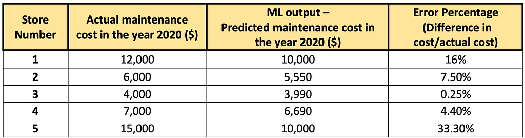 Table showing the error percentages of maintenance cost across various stores
As you can see, on an average, the ML model makes an error of 12 % while predicting the future costs (and the median error is around 8%).
Now that we have built the model and tested its performance, it’s time to get the predictions from the model for the next year, 2021. Suppose our model has predicted the below values for the next year.
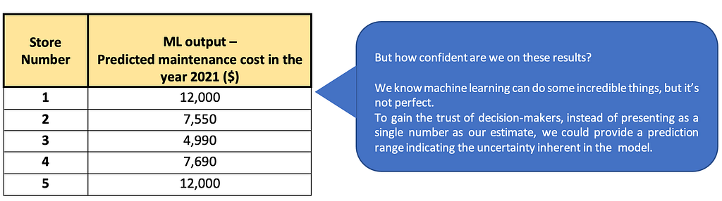
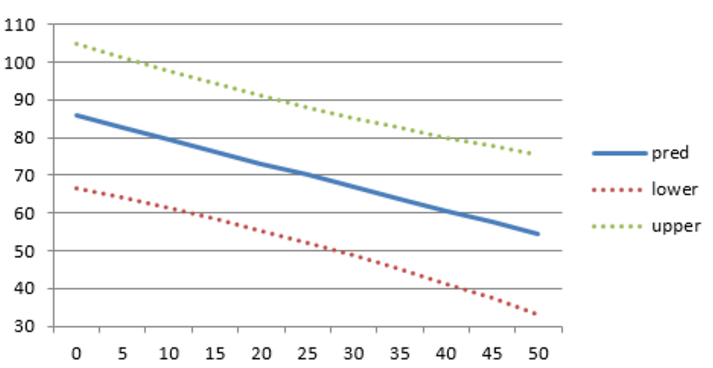
Something, as shown in the below table, would gain more trust on the predictions and will be more useful than a point prediction. Instead of predicting a single value for the maintenance cost, we are providing a range around these predictions.
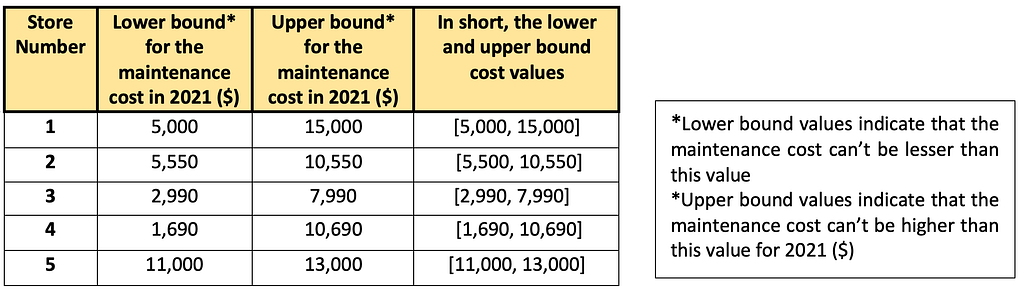 Table showing the upper and lower bounds
Along with the ranges, prediction intervals also provide a measure of confidence. A 95% confidence interval indicates that the model is 95% confident that the future maintenance cost of a given store falls within the calculated lower and upper bound. This will help the users to understand the uncertainty associated with every prediction. For example, the point prediction for store number 3 is 4990, and the calculated lower and upper bound range is [2990, 7990]. What this implies is that the predicted average maintenance cost is 4990 but with 95% confidence we can say that it will remain within the lower (2990) and upper (7990) bounds.
A wide prediction interval denotes that the model is not very confident about that prediction, while a narrow interval indicates that the model is very confident. Businesses can utilize this information to plan maintenance budgets more accurately and even decide to use the model results or some base maintenance value on the basis of the uncertainty associated with the predictions.
Prediction intervals can help data scientists to assess model performance as well. Even if model performance metrics (like MAPE and RMSE) are low, wider prediction intervals for all the predicted samples can indicate that the model has less conviction about these predictions. In such cases, additional measures can be taken to improve the model performance.
3. Machine Learning Approach to Generate Prediction Interval
To generate prediction intervals for any tree-based model (Random Forest and Gradient Boosting Model), we use Quantile Regressor Forest. To understand the concept of Quantile Regressor Forest better, let’s first understand the high-level working of Forest-based models.
Let’s say, we have trained a model to predict the maintenance cost of all refrigeration-related equipment in a store using the below feature information available as of 2018. The table below shows a mock training data.
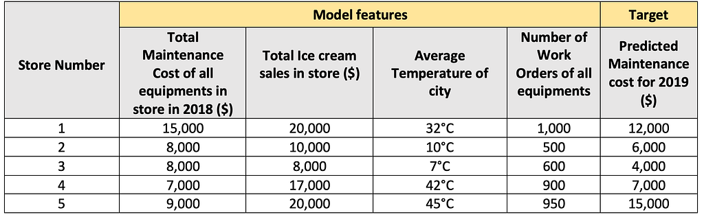 Training data
Please refer Random Forest and Gradient Boosting model to know more about their internal working.
The Forest model creates bins for all the features and calculates the average maintenance cost per bin. The below tables represent the bins for each feature and the average cost per bin.
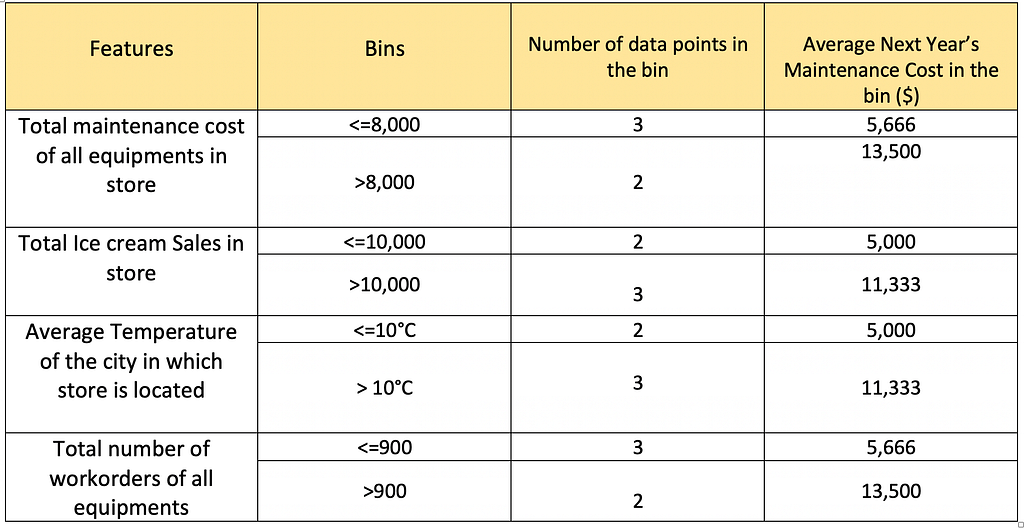 Table showing the working of forest-based models
Let’s say we want to predict the maintenance cost for stores 6 and 7 with the below feature values.
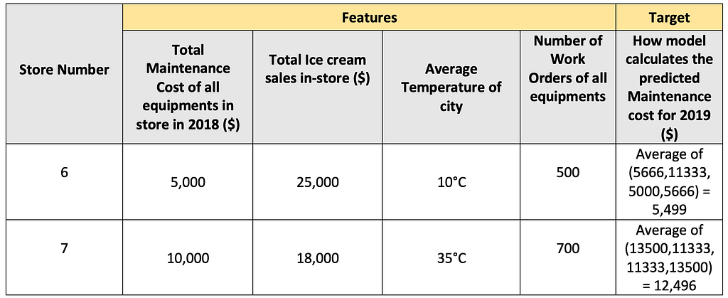 Table showing how the forest-based models predict for a new data point
- The model will first identify the bins corresponding to each feature value and the Average Next Year’s Maintenance Cost for that bin.
- It will then take the average of these Next Year’s Maintenance Costs for all the features, and this is the Next Year’s Maintenance Cost for that store
But we don’t know how certain the model is about these predictions. Here comes the advantage of Quantile Regressor Forest. They can generate prediction intervals using the concept of Quantiles.
Quantiles are a very common tool in Statistics to understand the distribution of a dataset. For e.g., if you want to know the value in your entire dataset which is higher than 25% of data points and lesser than 75% of data then you can calculate the 25% quantile. Similarly, we can calculate 95%, 5%, or any other quantile as per our requirement.
Let’s use the concept of quantiles in our model to expand its capability. Earlier the model was storing only the average maintenance cost per bin, but we can also store some other values per bin as below:
- Lowest Repair Cost with 5% of confidence: At least 95% of the data points which are falling into this bin has a higher cost than this.
- Highest Repair Cost with 95% of confidence: At least 95% of the data points which are falling into this bin has a lower cost than this.
This is how the data would look like with the updated capability.
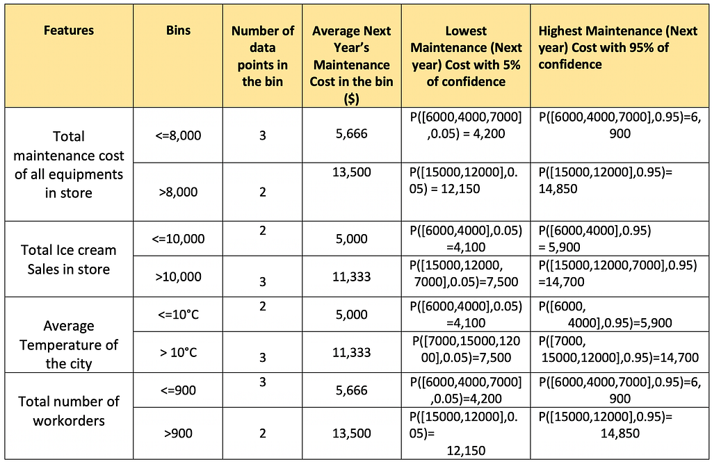 Table shows the calculation of the Lowest and Highest Maintenance repair costs. Here, P denotes Percentile()
Similarly, we can calculate the prediction intervals for the maintenance cost for stores 6 and 7 as shown below.
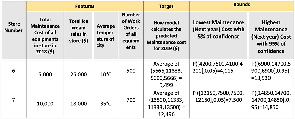 Table shows the calculation of Lowest and Highest Maintenance costs for a new data point
As we can see here, in the first data point, although the temperature was 10°C, the past year’s ice-cream sales were $25,000. Model understands this outlier behavior and that is why there is a significant difference between upper and lower bound values. Prediction intervals get wider as per uncertainty in model results.
In the next section, we can see how python sklearn libraries can help to generate these prediction intervals.
4. Python Implementation — Prediction Interval for GBM
Scikit learn’s GBM Model has inbuilt functionality to train Quantile Regressor Forest. It can be done by setting the parameter loss=quantile in the API call. The main difference is, instead of training 1 GBM model to predict the target, we need to train two additional GBM models as shown below:
- For the lower bound prediction, use
GradientBoostingRegressor(loss=‘quantile’, alpha=0.05)
- For the upper bound prediction, use
GradientBoostingRegressor(loss=‘quantile’, alpha=0.95)
At a high level, the model optimizes the loss function. By setting the loss parameter as quantile and choosing the appropriate alpha (quantile), we will be able to get the predictions corresponding to these percentiles. Thus, using these 3 models in conjunction, prediction intervals can be generated for every data point.
Let’s see this in action.
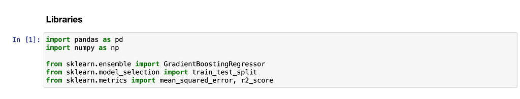 Required libraries
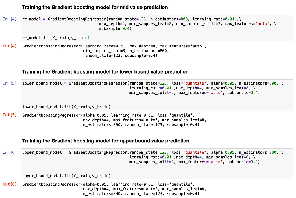 Training the 3 GBM models
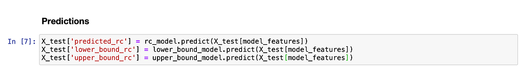 Making the predictions using the model
This is how we can use these 3 Models in conjunction to generate the prediction intervals for every data point.
5. Conclusion
Machine learning models are not perfect, therefore adding prediction intervals to the model output adds to its credibility. Quantile Regressor Forest is one of the many methods to do the same in a tree-based regression model. I hope this blog has given you a foundation in this concept and I encourage you to explore further and apply it to your own problems.
Written by :
- Achala Sharma(achala sharma) — Staff Data Scientist, Walmart Global Tech
- Bhavana Gopakumar (Bhavana G) — Data Scientist, Walmart Global Tech
6. References
Below are some references to generate prediction intervals for a variety of models
https://scikit-garden.github.io/examples/QuantileRegressionForests/
https://scikit-learn.org/dev/auto_examples/linear_model/plot_quantile_regression.html
https://datascienceplus.com/prediction-interval-the-wider-sister-of-confidence-interval/
Adding Prediction Intervals to Tree-based models was originally published in Walmart Global Tech Blog on Medium, where people are continuing the conversation by highlighting and responding to this story.
Article Link: Adding Prediction Intervals to Tree-based models | by Bhavana G | Walmart Global Tech Blog | Dec, 2021 | Medium